Modern Control Systems (MCS)
Modern Control Systems (MCS). Lecture-21-22-23 PID. Dr. Imtiaz Hussain Assistant Professor email: imtiaz.hussain@faculty.muet.edu.pk URL : http://imtiazhussainkalwar.weebly.com/. Lecture Outline. Introduction to PID Modes of Control On-Off Control Proportional Control

Modern Control Systems (MCS)
E N D
Presentation Transcript
Modern Control Systems (MCS) Lecture-21-22-23 PID Dr. Imtiaz Hussain Assistant Professor email: imtiaz.hussain@faculty.muet.edu.pk URL :http://imtiazhussainkalwar.weebly.com/
Lecture Outline • Introduction to PID • Modes of Control • On-Off Control • Proportional Control • Proportional + Integral Control • Proportional + Derivative Control • Proportional + Integral + Derivative Control • PID Tuning Rules • Zeigler-Nichol’s Tuning Rules • 1st Method • 2nd Method
Introduction • PID Stands for • P Proportional • I Integral • D Derivative
Introduction • The usefulness of PID controls lies in their general applicability to most control systems. • In particular, when the mathematical model of the plant is not known and therefore analytical design methods cannot be used, PID controls prove to be most useful. • In the field of process control systems, it is well known that the basic and modified PID control schemes have proved their usefulness in providing satisfactory control, although in many given situations they may not provide optimal control.
Introduction • It is interesting to note that more than half of the industrial controllers in use today are PID controllers or modified PID controllers. • Because most PID controllers are adjusted on-site, many different types of tuning rules have been proposed in the literature. • Using these tuning rules, delicate and fine tuning of PID controllers can be made on-site.
Four Modes of Controllers • Each mode of control has specific advantages and limitations. • On-Off (Bang Bang) Control • Proportional (P) • Proportional plus Integral (PI) • Proportional plus Derivative (PD) • Proportional plus Integral plus Derivative (PID)
On-Off Control • This is the simplest form of control. Set point Error Output
Proportional Control (P) • In proportional mode, there is a continuous linear relation between value of the controlled variable and position of the final control element. • Output of proportional controller is • The transfer function can be written as -
Proportional Controllers (P) • As the gain is increased the system responds faster to changes in set-point but becomes progressively underdamped and eventually unstable.
Proportional Plus Integral Controllers (PI) • Integral control describes a controller in which the output rate of change is dependent on the magnitude of the input. • Specifically, a smaller amplitude input causes a slower rate of change of the output.
Proportional Plus Integral Controllers (PI) • The major advantage of integral controllers is that they have the unique ability to return the controlled variable back to the exact set point following a disturbance. • Disadvantages of the integral control mode are that it responds relatively slowly to an error signal and that it can initially allow a large deviation at the instant the error is produced. • This can lead to system instability and cyclic operation. For this reason, the integral control mode is not normally used alone, but is combined with another control mode.
Proportional Plus Integral Control (PI) • The transfer function can be written as
Proportional Plus derivative Control (PD) • The transfer function can be written as
Proportional Plus derivative Control (PD) • The stability and overshoot problems that arise when a proportional controller is used at high gain can be mitigated by adding a term proportional to the time-derivative of the error signal. The value of the damping can be adjusted to achieve a critically damped response.
Proportional Plus derivative Control (PD) • The higher the error signal rate of change, the sooner the final control element is positioned to the desired value. • The added derivative action reduces initial overshoot of the measured variable, and therefore aids in stabilizing the process sooner. • This control mode is called proportional plus derivative (PD) control because the derivative section responds to the rate of change of the error signal
Proportional Plus Integral Plus Derivative Control (PID) + + - + ∫
Proportional Plus Integral Plus Derivative Control (PID) • Although PD control deals neatly with the overshoot and ringing problems associated with proportional control it does not cure the problem with the steady-state error. Fortunately it is possible to eliminate this while using relatively low gain by adding an integral term to the control function which becomes
CL RESPONSE RISE TIME OVERSHOOT SETTLING TIME S-S ERROR Kp Decrease Increase Small Change Decrease Ki Decrease Increase Increase Eliminate Kd Small Change Decrease Decrease Small Change The Characteristics of P, I, and D controllers
Tips for Designing a PID Controller • 1. Obtain an open-loop response and determine what needs to be improved • 2. Add a proportional control to improve the rise time • 3. Add a derivative control to improve the overshoot • 4. Add an integral control to eliminate the steady-state error • Adjust each of Kp, Ki, and Kd until you obtain a desired overall response. • Lastly, please keep in mind that you do not need to implement all three controllers (proportional, derivative, and integral) into a single system, if not necessary. For example, if a PI controller gives a good enough response (like the above example), then you don't need to implement derivative controller to the system. Keep the controller as simple as possible.
Part-II PID Tuning Rules
PID Tuning • The transfer function of PID controller is given as • It can be simplified as • Where
PID Tuning • The process of selecting the controller parameters () to meet given performance specifications is known as controller tuning. • Ziegler and Nichols suggested rules for tuning PID controllers experimentally. • Which are useful when mathematical models of plants are not known. • These rules can, of course, be applied to the design of systems with known mathematical models.
PID Tuning • Such rules suggest a set of values of that will give a stable operation of the system. • However, the resulting system may exhibit a large maximum overshoot in the step response, which is unacceptable. • In such a case we need series of fine tunings until an acceptable result is obtained. • In fact, the Ziegler–Nichols tuning rules give an educated guess for the parameter values and provide a starting point for fine tuning, rather than giving the final settings for in a single shot.
Zeigler-Nichol’s PID Tuning Methods • Ziegler and Nichols proposed rules for determining values of the based on the transient response characteristics of a given plant. • Such determination of the parameters of PID controllers or tuning of PID controllers can be made by engineers on-site by experiments on the plant. • There are two methods called Ziegler–Nichols tuning rules: • First method (open loop Method) • Second method (Closed Loop Method)
Zeigler-Nichol’s First Method • In the first method, we obtain experimentally the response of the plant to a unit-step input. • If the plant involves neither integrator(s) nor dominant complex-conjugate poles, then such a unit-step response curve may look S-shaped
Zeigler-Nichol’s First Method • This method applies if the response to a step input exhibits an S-shaped curve. • Such step-response curves may be generated experimentally or from a dynamic simulation of the plant. Table-1
Zeigler-Nichol’s Second Method • In the second method, we first set and . • Using the proportional control action only (as shown in figure), increase Kp from 0 to a critical value Kcrat which the output first exhibits sustained oscillations. • If the output does not exhibit sustained oscillations for whatever value Kp may take, then this method does not apply.
Zeigler-Nichol’s Second Method • Thus, the critical gain Kcr and the corresponding period Pcrare determined. Table-2
Example-1 1 t L
Example-2 • Consider the control system shown in following figure. • Apply a Ziegler–Nichols tuning rule for the determination of the values of parameters .
Example-2 • Transfer function of the plant is • Since plant has an integrator therefore Ziegler-Nichol’s first method is not applicable. • According to second method proportional gain is varied till sustained oscillations are produced. • That value of Kc is referred as Kcr.
Example-2 • Here, since the transfer function of the plant is known we can find using • Root Locus • Routh-Herwitz Stability Criterion • By setting and closed loop transfer function is obtained as follows.
Example-2 • The value of that makes the system marginally unstable so that sustained oscillation occurs can be obtained as • The Routh array is obtained as • Examining the coefficients of first column of the Routh array we find that sustained oscillations will occur if . • Thus the critical gain is
Example-2 • With gain set equal to 30, the characteristic equation becomes • To find the frequency of sustained oscillations, we substitute into the characteristic equation. • Further simplification leads to
Example-2 • Hence the period of sustained oscillations is • Referring to Table-2 5
Example-2 5 • Transfer function of PID controller is thus obtained as
Electronic PID Controller • In terms of Kp, Ki, Kd we have
To download this lecture visit http://imtiazhussainkalwar.weebly.com/ End of Lecture-21-22-23