
MATLAB Matrix Operations: Basics, Exercises, and Display Techniques
This guide provides a comprehensive overview of basic matrix operations in MATLAB, including matrix initialization, joining matrices, and using the colon operator. Learn how to manipulate arrays, perform element-wise calculations, and utilize built-in functions for effective data handling. Additionally, the document outlines exercises for practical application, demonstrating how to extract subarrays and display results using various methods such as `disp()` and `fprintf()`. Enhance your MATLAB skills with practical examples that focus on array and matrix arithmetic.

MATLAB Matrix Operations: Basics, Exercises, and Display Techniques
E N D
Presentation Transcript
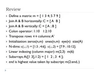
Review • Define a matrix: m = [ 1 3 4; 5 7 9 ] • Join A & B horizontally: C = [ A B ] • Join A & B vertically: C = [ A ; B ] • Colon operator: 1:10 1:2:10 • Transpose rows ↔ columns: A’ • Initialization: zeros(n,m) ones(n,m) eye(n) size(A) • N-dims: c(:,:,1) = [1:3 ; 4:6]; c(:,:,2) = [7:9 ; 10:12]; • Linear indexing (column major): m(2,3) m(6) • Subarrays: A([1 3],1:2) = [ 1 2 ; 3 4 ]; • end is highest value taken by subscript: m(2:end,:)
Exercises • Create the following matrix c using the colon operator: Now display the following subarrays: • (a) the 2nd row • (b) the last column • (c) 1st and 2nd rows from the 2nd column onwards • (d) the 6th element (using single subscript) • (e) all elements from the 4th onwards • (f) 1st and 2nd rows (2nd and 4th columns only) • (g) 1st and 3rd rows, 2nd column only • (h) a new 2x4 matrix with row 3 on both of its rows c(2,:) c(:,end) c(1:2,2:end) c(6) c(4:end) c(1:2,[2 4]) c([1 3],2) c([3 3],:)
Displaying output The simplest way to display output is simply to omit the semi-colon at the end of the line Another way is to use disp(), possibly in combination with num2str() or int2str() • disp(pi) • str = [‘The value of pi = ’,num2str(pi)] • disp(str) For more tailored output use the fprintf function: • General syntax is fprintf(format,data), e.g. • fprintf(‘The value of pi is %f \n’,pi) • fprintf(‘The value of pi is %6.2f \n’,pi) • You can also use: • %d Display as an integer • %e Display in exponential format • %g Either floating point of exponential format (the shorter) • \t , \n Tab separator and new line
Data files using load/save Probably the easiest way to import data into a Matlab program is from a tab delimited file. Excel can export tables in tab-delimited format. These can be read using the load function with the -ascii option Example: Create a table as follows using an Open Office Calc spreadsheet and save it as tab-delimited Open Office:File – Save as – Format CSV. Tick Edit Filter settings and change delimiter to <TAB> Excel: File – Save As Type “Text (Tab delimited) (*.txt)“ If you open the file in Text Editor, it should look like this: 12 23 34 45 56 67 78 89
Data files using load/save • x = load(‘-ascii’,’my.tab.delimited.file.csv’) • x = • 12 23 34 45 • 56 67 78 89 • Similarly, one can use the save function to store in ascii format (we will look at other I/O later): • x = [1:3;4:6]; • save(‘-ascii’,’xout.dat’,’x’) • The resulting file looks like this: 1.00000000e+000 2.00000000e+000 3.00000000e+000 4.00000000e+000 5.00000000e+000 6.00000000e+000
Scalar arithmetic Assigment statements are of the form • variable_name = expression • Scalar operators: • Addition, subtraction: a+b a-b • Multiplication, division: a*b a/b • Exponentiation: a^b When many operations are combined into a single expression, it is important to know in what order Matlab will evaluate the terms.
Scalar arithmetic Matlab has a series of rules governing the hierarchy (or order) in which operations are evaluated within an expression, as follows • 1. Expressions in parentheses (innermost to outermost) • 2. Exponentials (left to right) • 3. Multiplications and divisions (left to right) • 4. Additions and subtractions (left to right) Thus, the expression • distance = 0.5 * accel * time ^ 2 • is equivalent to • distance = 0.5 * accel * (time ^ 2) • but not equivalent to • distance = (0.5 * accel * time) ^ 2
Exercise • Declare: a=3; b=2; c=5; d=3 and calculate the following expressions:
Array and Matrix operations • Matlab has two types of operations between arrays: • (a) element-by-element operations where the two operands have the same number of rows and columns, for example • A = [1 2 ; 3 4]; B=[-1 3; -2 1] • Addition, Subtraction: A+B A-B • Multiplication, Division: A .* B A ./ B • Exponentiation: A .^ B • One operand can be scalar, the other a matrix • e.g. 2 .^ A • Although for multiplication,divsion A * 2 = A .* 2 and A/2 = A./2 • (b) Matrix operations • Ordinary matrix multiplication: A * B • Matrix exponent: A^2 (scalar exponent) • Matrix left division: A \ B = inv(A) * b
Exercise • If a= ,b= ,c= • Calculate: • a + b • a X c • c X a (should give error!) • Elementwise a X b • Matrix multiplication: a X b • a X a X a X a • If x = 1:10 and y=ones(1,10) • Calculate (remember that z x zT = )
Common built-in functions • Mathematical functions: • sum(x): sum of elements of a vector or columns of a matrix • mean(x): mean, similarly columnwise for matrix • rand, rand(m), rand(m,n): random numbers (uniform, interval [0,1]) • abs(x) • sin(x), cos(x), tan(x) • exp(x), log(x), log10(x) • [value,index] = max(x), [value,index] = min(x) • sqrt(x) • Rounding • ceil(x), floor(x): to +∞ and -∞ respectively • fix(x): nearest integer towards zero • round(x): to nearest integer • String conversion • int2str, num2str, str2num
Exercises • Assign n=100, then compute • Compute: • Compute (using sum then without sum) • if x=3, calculate cosh (using exp) • Generate a vector r of means for 1000 random number vectors of length 50. See your results with the command: hist(r,40)


