Download
1 / 21
210 likes | 349 Vues
Section 4.3 ~ Measures of Variation. Introduction to Probability and Statistics Ms. Young. Objective. Sec. 4.3. In this section you will be able to understand and interpret the following common measures of variation: Range The five-number summary (boxplot or box-and-whisker plot)

E N D
Section 4.3 ~ Measures of Variation Introduction to Probability and Statistics Ms. Young
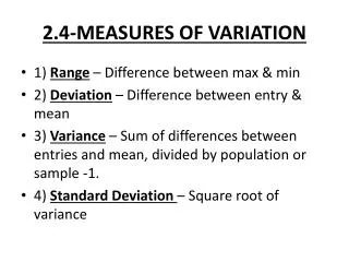
Objective Sec. 4.3 • In this section you will be able to understand and interpret the following common measures of variation: • Range • The five-number summary (boxplot or box-and-whisker plot) • Standard deviation
Sec. 4.3 Range • Recall that the variation of a data set describes how widely data are spread out about the center of the data set (low, moderate, or high) • The range of a data set is the difference between its highest and lowest data values • Example ~ the following data represents the wait time (in minutes) for 11 customers at two different banks Big Bank: 4.1 5.2 5.6 6.2 6.7 7.2 7.7 7.7 8.5 9.3 11.0 Best Bank: 6.6 6.7 6.7 6.9 7.1 7.2 7.3 7.4 7.7 7.8 7.8 The range for Big Bank is 11.0 – 4.1 = 6.9 minutes The range for Best Bank is 7.8 – 6.6 = 1.2 minutes Since the range for Big Bank is much larger, this tells us that is has a higher variation (spread out wider)
Sec. 4.3 Example 1 • Computing the range can be useful at times, but can also be misleading • Example ~ Consider the following data sets which represent the quiz scores for nine students. Which set has the greater range? Would you also say that this set has the greater variation? Quiz 1: 1 10 10 10 10 10 10 10 10 Quiz 2: 2 3 4 5 6 7 8 9 10 The range for quiz 1 is 10 – 1 = 9 points The range for quiz 2 is 10 – 2 = 8 points Quiz 1 has a higher range, but aside from the single outlier is has no variation at all, therefore quiz 2 has the greater variation
Sec. 4.3 Quartiles • Quartiles are values that divide the data distribution into quarters • There are three quartiles, lower (Q1), middle (Q2), and upper (Q3) • In order to find the quartiles, the values must be in ascending order
Sec. 4.3 Lower Quartile • The lower quartile (Q1) is the median of the values in the lower half of the data set • If the data set is odd, exclude the middle value • Ex. ~ 4.1 5.2 5.6 6.2 6.7 7.2 7.7 7.7 8.5 9.3 11.0 • If the data set is even, split in half • Ex. ~ Q1 6.6 6.7 6.7 6.9 7.1 7.2 7.3 7.4 7.7 7.8 Q1
Sec. 4.3 Middle Quartile • The middle quartile (Q2) is the overall median of the data set • Odd data set: • Ex. ~ 4.1 5.2 5.6 6.2 6.7 7.2 7.7 7.7 8.5 9.3 11.0 • Even data set: • Ex. ~ Q2 6.6 6.7 6.7 6.9 7.1 7.2 7.3 7.4 7.7 7.8 Q2
Sec. 4.3 Upper Quartile • The upper quartile (Q3) is the median of the values in the upper half of the data set • If the data set is odd, exclude the middle value • Ex. ~ 4.1 5.2 5.6 6.2 6.7 7.2 7.7 7.7 8.5 9.3 11.0 • If the data set is even, split in half • Ex. ~ Q3 6.6 6.7 6.7 6.9 7.1 7.2 7.3 7.4 7.7 7.8 Q3
Sec. 4.3 Five-Number Summary • Once you know the quartiles, you can describe a distribution with a five-number summary, consisting of the low value, lower quartile, median (middle quartile), upper quartile, and high value • Ex. ~ Write the five number summaries for the waiting times for Big Bank and Best Bank.
Sec. 4.3 Boxplots • The five-number summary can be displayed with a graph called a boxplot (or box-and-whisker plot) • The values from the lower to upper quartiles are enclosed in a box and a line extends from the box to the low and high values which are considered the whiskers • Steps to Drawing a Boxplot • Step 1: Draw a number line that spans all the data values in the data set (usually leaving room on either end of the high and low values) • Step 2: Enclose the values from the lower to the upper quartile in a box • Step 3: Draw a vertical line through the box at the median • Step 4: Add “whiskers” by extending to the low and high values
Sec. 4.3 Example 2 • A bakery collected the following data about the number of loaves of fresh bread sold on each of 10 business days. Write a five-number summary and then make a boxplot to represent this data. State any skewness. 43 39 17 38 50 42 34 8 39 43
Sec. 4.3 Percentiles • Percentiles divide a data set into 100 segments • They are essentially a rank of each individual data value • The nth percentile of a data set divides the bottom n% of data values from the top (100-n)% • Example ~ The 35th percentile of a data set is the value that separates the bottom 35% of data values from the top 65% • If exam results stated that your exam score is in the 35th percentile, that means that you scored higher than 35% of the people that took the exam and lower than 65% of the people that took the exam • If a data value lies between two percentiles it is often said to lie in the lower of the two percentiles • Example ~ If you score higher than 84.7% of all people taking a college entrance examination, it is said that you scored in the 84th percentile • The percentile of a data value is found using the following formula:
Sec. 4.3 Percentiles Cont’d… • Example ~ What percentile is the lower value, Q1 , Q2 , Q3 , and the upper value in for Big Bank? • Lower value = 4.1; there are no values lower than 4.1, so it is in the 0th percentile (0/11 = 0) • Q1 = 5.6; there are two values lower than 5.6 in a set of eleven values, so it is in the 18th percentile (2/11 = .1818…) • Q2 = 7.2; there are five values lower than 7.2 in a set of eleven values, so it is in the 45th percentile (5/11 = .4545…) • Q3 = 8.5; there are eight values lower than 8.5 in a set of eleven values, so it is in the 72nd percentile (8/11 = .7272…) • Upper value = 11.0; there are ten values lower than 11.0 in a set of eleven values, so it is in the 90th percentile (10/11 = .9090…)
Sec. 4.3 Example 3 • Refer to table 4.4 on p.168 to answer the following questions. • What is the percentile for the data value of 592.79 ng/ml for smokers? • Since this is the 47th value, there are 46 values falling below which means it will fall in the 92nd percentile (46/50 = .92) • What values mark the 36th percentile in the data set on p.168? • Because we know that there are a total of 50 values in the set, we can set up an equation to solve for the value • This means that the 18th value in the data set marks the 36th percentile, therefore 20.16 ng/ml (smokers) and 0.33 ng/ml (nonsmokers)
Sec. 4.3 Standard Deviation • While the range and a five-number summary are both methods of explaining variation, the standard deviation is a single number that is most commonly used to describe variation of a data set • This is universally accepted as the best measure of variation for a statistical distribution • The standard deviation is found by averaging the deviation from each data value to the mean • To calculate the standard deviation for a data set, follow these steps: • 1. Compute the mean of the data set • 2. Find the deviation of each data value from the mean Deviation from mean = data value – mean • 3. Find the squares of all the deviations • 4. Add all the squares • 5. Divide this sum by the total number of data values minus 1 • 6. Take the square root of the value found in step 5 • In general, the formula for the standard deviation is:
Sec. 4.3 Example 4 Find the standard deviation of the following data set. 1 5 6 8 11 Step 1: Find the mean Step 2: Find the deviations from the mean 1 – 6.2 = -5.2 5 – 6.2 = -1.2 6 – 6.2 = -0.2 8 – 6.2 = 1.8 11 – 6.2 = 4.8 Step 3: Square the deviations (-5.2)²= 27.04 (-1.2)²= 1.44 (-0.2)² = .04 (1.8)²= 3.24 (4.8)²= 23.04
Sec. 4.3 Example 4 Cont’d… Step 4: Add the squares 27.04 + 1.44 + .04 + 3.24 + 23.04 = 54.8 Step 5: Divide the sum by the total number of data values – 1 54.8/(5 – 1) = 54.8/4 = 13.7 Step 6: Take the square root of the value in step 5 The standard deviation is 3.7. This means that most values occur within 3.7 units in either direction of the mean of 6.2.
Sec. 4.3 The Range Rule of Thumb • The range rule of thumb is an approximation of the standard deviation • Example ~ Estimate the standard deviation of the data set used in the last example. 1 5 6 8 11 This approximation is not the best estimate in comparison to the actual standard deviation of 3.7, but is a rough estimate. It would be a much better representation if the data values were closer in number. • If you know the standard deviation of a data set, you can use the range rule of thumb to estimate the high and low values of a data set:
Sec. 4.3 Example 5 • Use the range rule of thumb to estimate the standard deviations for the waiting times at Big Bank and Best Bank. Compare the estimates to the actual values in example 4 in the book (p.172). • Big Bank: • Best Bank: • The actual standard deviations in example 4 are 1.96 and .44 respectively, so the range rule of thumb in in the right ballpark, but slightly underestimates it
Sec. 4.3 Example 6 • Studies of the gas mileage of a BMW under varying driving conditions show that it gets a mean of 22 miles per gallon with a standard deviation of 3 miles per gallon. Estimate the minimum and maximum typical gas mileage amounts that you can expect under ordinary driving conditions. The range of gas mileage for the car is roughly from 16 to 28 miles per gallon.
Sec. 4.3 Standard Deviation Using Summation Notation Recall from section 4.1, the notations used to describe mean: The standard deviation formula using summation notation is as follows: