Download
1 / 63
630 likes | 833 Vues
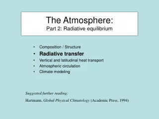
Radiative Transfer in the Atmosphere. Lectures in Benevento June 2007 Paul Menzel UW/CIMSS/AOS. Using wavelengths c 2 / λ T Planck’s Law B( λ ,T) = c 1 / λ 5 / [e -1] (mW/m 2 /ster/ c m) where λ = wavelengths in cm

E N D
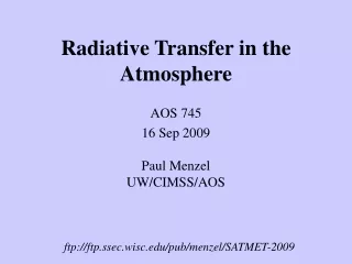
Radiative Transfer in the Atmosphere Lectures in Benevento June 2007 Paul MenzelUW/CIMSS/AOS
Using wavelengths c2/λT Planck’s Law B(λ,T) = c1 / λ5 / [e -1] (mW/m2/ster/cm) where λ = wavelengths in cm T = temperature of emitting surface (deg K) c1 = 1.191044 x 10⁻⁵ (mW/m2/ster/cm-4) c2 = 1.438769 (cm deg K) Wien's Law dB(λmax,T) / dλ = 0 where λ(max) = .2897/T indicates peak of Planck function curve shifts to shorter wavelengths (greater wavenumbers) with temperature increase. Note B(λmax,T) ~ T5. Stefan-Boltzmann Law E = B(λ,T) dλ = T4, where = 5.67 x 10⁻⁸ W/m2/deg4. o states that irradiance of a black body (area under Planck curve) is proportional to T4 . Brightness Temperature c 1 T = c2 / [λln( _____ + 1)] is determined by inverting Planck functionλ5Bλ
Spectral Distribution of Energy Radiated from Blackbodies at Various Temperatures
Temperature Sensitivity of B(λ,T) for typical earth scene temperatures B (λ, T) / B (λ, 273K) 4μm 6.7μm 2 1 10μm 15μm microwave • 250 300 • Temperature (K)
Spectral Characteristics of Energy Sources and Sensing Systems
Normalized black body spectra representative of the sun (left) and earth (right), plotted on a logarithmic wavelength scale. The ordinate is multiplied by wavelength so that the area under the curves is proportional to irradiance.
Relevant Material in Applications of Meteorological Satellites CHAPTER 2 - NATURE OF RADIATION 2.1 Remote Sensing of Radiation 2-1 2.2 Basic Units 2-1 2.3 Definitions of Radiation 2-2 2.5 Related Derivations 2-5 CHAPTER 3 - ABSORPTION, EMISSION, REFLECTION, AND SCATTERING 3.1 Absorption and Emission 3-1 3.2 Conservation of Energy 3-1 3.3 Planetary Albedo 3-2 3.4 Selective Absorption and Emission 3-2 3.7 Summary of Interactions between Radiation and Matter 3-6 3.8 Beer's Law and Schwarzchild's Equation 3-7 3.9 Atmospheric Scattering 3-9 3.10 The Solar Spectrum 3-11 3.11 Composition of the Earth's Atmosphere 3-11 3.12 Atmospheric Absorption and Emission of Solar Radiation 3-11 3.13 Atmospheric Absorption and Emission of Thermal Radiation 3-12 3.14 Atmospheric Absorption Bands in the IR Spectrum 3-13 3.15 Atmospheric Absorption Bands in the Microwave Spectrum 3-14 3.16 Remote Sensing Regions 3-14 CHAPTER 5 - THE RADIATIVE TRANSFER EQUATION (RTE) 5.1 Derivation of RTE 5-1 5.10 Microwave Form of RTE 5-28
Emission, Absorption, Reflection, and Scattering Blackbody radiation B represents the upper limit to the amount of radiation that a real substance may emit at a given temperature for a given wavelength. Emissivity is defined as the fraction of emitted radiation R to Blackbody radiation, = R /B . In a medium at thermal equilibrium, what is absorbed is emitted (what goes in comes out) so a = . Thus, materials which are strong absorbers at a given wavelength are also strong emitters at that wavelength; similarly weak absorbers are weak emitters. If a, r, and represent the fractional absorption, reflectance, and transmittance, respectively, then conservation of energy says a + r + = 1 . For a blackbody a = 1, it follows that r = 0 and = 0 for blackbody radiation. Also, for a perfect window = 1, a = 0 and r = 0. For any opaque surface = 0, so radiation is either absorbed or reflected a + r = 1. At any wavelength, strong reflectors are weak absorbers (i.e., snow at visible wavelengths), and weak reflectors are strong absorbers (i.e., asphalt at visible wavelengths).
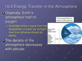
Planetary Albedo • Planetary albedo is defined as the fraction of the total incident solar irradiance, S, that is reflected back into space. Radiation balance then requires that the absorbed solar irradiance is given by • E = (1 - A) S/4. • The factor of one-fourth arises because the cross sectional area of the earth disc to solar radiation, r2, is one-fourth the earth radiating surface, 4r2. Thus recalling that S = 1380 Wm-2, if the earth albedo is 30 percent, • then E = 241 Wm-2.
Selective Absorption and Transmission Assume that the earth behaves like a blackbody and that the atmosphere has an absorptivity aS for incoming solar radiation and aL for outgoing longwave radiation. Let Ya be the irradiance emitted by the atmosphere (both upward and downward); Ys the irradiance emitted from the earth's surface; and E the solar irradiance absorbed by the earth-atmosphere system. Then, radiative equilibrium requires E - (1-aL) Ys - Ya = 0 , at the top of the atmosphere, (1-aS) E - Ys + Ya = 0 , at the surface. Solving yields (2-aS) Ys = E , and (2-aL) (2-aL) - (1-aL)(2-aS) Ya = E . (2-aL) Since aL > aS, the irradiance and hence the radiative equilibrium temperature at the earth surface is increased by the presence of the atmosphere. With aL = .8 and aS = .1 and E = 241 Wm-2, Stefans Law yields a blackbody temperature at the surface of 286 K, in contrast to the 255 K it would be if the atmospheric absorptance was independent of wavelength (aS = aL). The atmospheric gray body temperature in this example turns out to be 245 K.
Incoming Outgoing IR solar • E (1-al)Ys Ya top of the atmosphere • (1-as)E Ys Ya earth surface. (2-aS) Ys = E = Ts4 (2-aL)
Expanding on the previous example, let the atmosphere be represented by two layers and let us compute the vertical profile of radiative equilibrium temperature. For simplicity in our two layer atmosphere, let aS = 0 and aL = a = .5, u indicate upper layer, l indicate lower layer, and s denote the earth surface. Schematically we have: E (1-a)2Ys (1-a)Yl Yu top of the atmosphere E (1-a)Ys Yl Yu middle of the atmosphere E Ys Yl(1-a)Yu earth surface. Radiative equilibrium at each surface requires E = .25 Ys + .5 Yl + Yu , E = .5 Ys + Yl - Yu , E = Ys - Yl - .5 Yu . Solving yields Ys = 1.6 E, Yl = .5 E and Yu = .33 E. The radiative equilibrium temperatures (blackbody at the surface and gray body in the atmosphere) are readily computed. Ts = [1.6E / σ]1/4 = 287 K , Tl = [0.5E / 0.5σ]1/4 = 255 K , Tu = [0.33E / 0.5σ]1/4 = 231 K . Thus, a crude temperature profile emerges for this simple two-layer model of the atmosphere.
Transmittance Transmission through an absorbing medium for a given wavelength is governed by the number of intervening absorbing molecules (path length u) and their absorbing power (k) at that wavelength. Beer’s law indicates that transmittance decays exponentially with increasing path length - ku (z) (z ) = e where the path length is given by u (z) = dz . z ku is a measure of the cumulative depletion that the beam of radiation has experienced as a result of its passage through the layer and is often called the optical depth . Realizing that the hydrostatic equation implies g dz = - q dp where q is the mixing ratio and is the density of the atmosphere, then p - ku (p) u (p) = q g-1 dp and (p o ) = e . o
Spectral Characteristics of Atmospheric Transmission and Sensing Systems
Aerosol Size Distribution • There are 3 modes : • - « nucleation »: radius is between 0.002 and 0.05 mm. They result from combustion processes, photo-chemical reactions, etc. • - « accumulation »: radius is between 0.05 mmand 0.5 mm. Coagulation processes. • - « coarse »: larger than 1 mm. From mechanical processes like aeolian erosion. • « fine » particles (nucleation and accumulation) result from anthropogenic activities, coarse particles come from natural processes. 0.01 0.1 1.0 10.0
Measurements in the Solar Reflected Spectrum across the region covered by AVIRIS
AVIRIS Movie #1 AVIRIS Image - Linden CA 20-Aug-1992 224 Spectral Bands: 0.4 - 2.5 mm Pixel: 20mx 20mScene: 10km x 10km
AVIRIS Movie #2 AVIRIS Image - Porto Nacional, Brazil 20-Aug-1995 224 Spectral Bands: 0.4 - 2.5 mm Pixel: 20mx 20mScene: 10km x 10km
Relevant Material in Applications of Meteorological Satellites CHAPTER 2 - NATURE OF RADIATION 2.1 Remote Sensing of Radiation 2-1 2.2 Basic Units 2-1 2.3 Definitions of Radiation 2-2 2.5 Related Derivations 2-5 CHAPTER 3 - ABSORPTION, EMISSION, REFLECTION, AND SCATTERING 3.1 Absorption and Emission 3-1 3.2 Conservation of Energy 3-1 3.3 Planetary Albedo 3-2 3.4 Selective Absorption and Emission 3-2 3.7 Summary of Interactions between Radiation and Matter 3-6 3.8 Beer's Law and Schwarzchild's Equation 3-7 3.9 Atmospheric Scattering 3-9 3.10 The Solar Spectrum 3-11 3.11 Composition of the Earth's Atmosphere 3-11 3.12 Atmospheric Absorption and Emission of Solar Radiation 3-11 3.13 Atmospheric Absorption and Emission of Thermal Radiation 3-12 3.14 Atmospheric Absorption Bands in the IR Spectrum 3-13 3.15 Atmospheric Absorption Bands in the Microwave Spectrum 3-14 3.16 Remote Sensing Regions 3-14 CHAPTER 5 - THE RADIATIVE TRANSFER EQUATION (RTE) 5.1 Derivation of RTE 5-1 5.10 Microwave Form of RTE 5-28
Radiative Transfer Equation The radiance leaving the earth-atmosphere system sensed by a satellite borne radiometer is the sum of radiation emissions from the earth-surface and each atmospheric level that are transmitted to the top of the atmosphere. Considering the earth's surface to be a blackbody emitter (emissivity equal to unity), the upwelling radiance intensity, I, for a cloudless atmosphere is given by the expression I = sfc B( Tsfc) (sfc - top) + layer B( Tlayer) (layer - top) layers where the first term is the surface contribution and the second term is the atmospheric contribution to the radiance to space.
Rsfc R1 R2 top of the atmosphere τ2=transmittance of upper layer of atm τ1= transmittance of lower layer of atm bb earth surface. Robs = Rsfc τ1 τ2 + R1 (1-τ1) τ2 + R2 (1- τ2)
In standard notation, I = sfc B(T(ps)) (ps) + (p) B(T(p)) (p) p The emissivity of an infinitesimal layer of the atmosphere at pressure p is equal to the absorptance (one minus the transmittance of the layer). Consequently, (p) (p) = [1 - (p)] (p) Since transmittance is an exponential function of depth of absorbing constituent, p+p p (p) (p) = exp [ - k q g-1 dp] * exp [ - k q g-1 dp] = (p + p) p o Therefore (p) (p) = (p) - (p + p) = - (p) . So we can write I = sfc B(T(ps)) (ps) - B(T(p)) (p) . p which when written in integral form reads ps I = sfc B(T(ps)) (ps) - B(T(p)) [ d(p) / dp ] dp . o
When reflection from the earth surface is also considered, the Radiative Transfer Equation for infrared radiation can be written o I = sfc B(Ts) (ps) + B(T(p)) F(p) [d(p)/ dp] dp ps where F(p) = { 1 + (1 - ) [(ps) / (p)]2 } The first term is the spectral radiance emitted by the surface and attenuated by the atmosphere, often called the boundary term and the second term is the spectral radiance emitted to space by the atmosphere directly or by reflection from the earth surface. The atmospheric contribution is the weighted sum of the Planck radiance contribution from each layer, where the weighting function is [ d(p) / dp ]. This weighting function is an indication of where in the atmosphere the majority of the radiation for a given spectral band comes from.
Schwarzchild's equation At wavelengths of terrestrial radiation, absorption and emission are equally important and must be considered simultaneously. Absorption of terrestrial radiation along an upward path through the atmosphere is described by the relation -dLλabs = Lλ kλ ρ sec φ dz . Making use of Kirchhoff's law it is possible to write an analogous expression for the emission, dLλem = Bλ dλ = Bλ daλ = Bλ kλ ρ sec φ dz , where Bλ is the blackbody monochromatic radiance specified by Planck's law. Together dLλ = - (Lλ - Bλ) kλ ρ sec φ dz . This expression, known as Schwarzchild's equation, is the basis for computations of the transfer of infrared radiation.
Schwarzschild to RTE dLλ = - (Lλ - Bλ) kλ ρ dz but d = kρdz since = exp [- k ρ dz]. z so dLλ= - (Lλ - Bλ) d dLλ+ Lλ d = Bλd d (Lλ ) = Bλd Integrate from 0 to Lλ ( ) ( ) - Lλ (0 ) (0 ) = Bλ [d /dz] dz. 0 and Lλ (sat) = Lλ (sfc) (sfc) + Bλ [d /dz] dz. 0
Earth emitted spectra overlaid on Planck function envelopes O3 CO2 H20 CO2
Weighting Functions Longwave CO2 14.7 1 680 CO2, strat temp 14.4 2 696 CO2, strat temp 14.1 3 711 CO2, upper trop temp 13.9 4 733 CO2, mid trop temp 13.4 5 748 CO2, lower trop temp 12.7 6 790 H2O, lower trop moisture 12.0 7 832 H2O, dirty window Midwave H2O & O3 11.0 8 907 window 9.7 9 1030 O3, strat ozone 7.4 10 1345 H2O, lower mid trop moisture 7.0 11 1425 H2O, mid trop moisture 6.5 12 1535 H2O, upper trop moisture
line broadening with pressure helps to explain weighting functions ABC High Mid Low A B C ABC
CO2 channels see to different levels in the atmosphere 14.2 um 13.9 um 13.6 um 13.3 um
These water vapor weighting functions reflect the radiance sensitivity of the specific channels to a water vapor % change at a specific level (equivalent to dR/dlnq scaled by dlnp). Moisture Weighting Functions Pressure Weighting Function Amplitude Wavenumber (cm-1) UW/CIMSS The advanced sounder has more and sharper weighting functions
Characteristics of RTE * Radiance arises from deep and overlapping layers * The radiance observations are not independent * There is no unique relation between the spectrum of the outgoing radiance and T(p) or Q(p) * T(p) is buried in an exponent in the denominator in the integral * Q(p) is implicit in the transmittance * Boundary conditions are necessary for a solution; the better the first guess the better the final solution
To investigate the RTE further consider the atmospheric contribution to the radiance to space of an infinitesimal layer of the atmosphere at height z, dIλ(z) = Bλ(T(z)) dλ(z) . Assume a well-mixed isothermal atmosphere where the density drops off exponentially with height ρ = ρo exp ( - z), and assume kλ is independent of height, so that the optical depth can be written for normal incidence σλ = kλ ρ dz = -1 kλ ρo exp( - z) z and the derivative with respect to height dσλ = - kλ ρo exp( - z) = - σλ . dz Therefore, we may obtain an expression for the detected radiance per unit thickness of the layer as a function of optical depth, dIλ(z) dλ(z) = Bλ(Tconst) = Bλ(Tconst) σλ exp (-σλ) . dz dz The level which is emitting the most detected radiance is given by d dIλ(z) {} = 0 , or where σλ = 1. dz dz Most of monochromatic radiance detected is emitted by layers near level of unit optical depth.
Profile Retrieval from Sounder Radiances ps I = sfc B(T(ps)) (ps) - B(T(p)) F(p) [ d(p) / dp ] dp . o I1, I2, I3, .... , In are measured with the sounder P(sfc) and T(sfc) come from ground based conventional observations (p) are calculated with physics models (using for CO2 and O3) sfc is estimated from a priori information (or regression guess) First guess solution is inferred from (1) in situ radiosonde reports, (2) model prediction, or (3) blending of (1) and (2) Profile retrieval from perturbing guess to match measured sounder radiances
GOES-12 Sounder – Brightness Temperature (Radiances) – 12 bands
Sounder Retrieval Products • ps • I = (sfc) B(T(ps)) (ps) - B(T(p)) F(p) [ d(p) / dp ] dp . • o • Direct • brightness temperatures • Derived in Clear Sky • 20 retrieved temperatures (at mandatory levels) • 20 geo-potential heights (at mandatory levels) • 11 dewpoint temperatures (at 300 hPa and below) • 3 thermal gradient winds (at 700, 500, 400 hPa) • 1 total precipitable water vapor • 1 surface skin temperature • 2 stability index (lifted index, CAPE) • Derived in Cloudy conditions • 3 cloud parameters (amount, cloud top pressure, and cloud top temperature) • Mandatory Levels (in hPa) • sfc 780 300 70 • 1000 700 250 50 • 950 670 200 30 • 920 500 150 20 • 850 400 100 10
BT differences resulting from 10 ppmv change in CO2 concentration
Microwave RTE Lectures in Benevento June 2007 Paul MenzelUW/CIMSS/AOS