Introduction to radiative transfer
Introduction to radiative transfer. Robert Hudson. Electromagnetic spectrum. Schematic of a wave. WAVELENGTH. DISTANCE BETWEEN SUCCESSIVE PEAKS GIVEN THE SYMBOL λ MANY UNITS USED : (A) MICRON, 10 -6 METERS (B) NANOMETER, 10 -9 METERS (C) ANGSTROM, 10 -10 METERS. FREQUENCY.

Introduction to radiative transfer
E N D
Presentation Transcript
Introduction to radiative transfer Robert Hudson
WAVELENGTH • DISTANCE BETWEEN SUCCESSIVE PEAKS • GIVEN THE SYMBOL λ • MANY UNITS USED : • (A) MICRON, 10-6 METERS • (B) NANOMETER, 10-9 METERS • (C) ANGSTROM, 10-10 METERS
VELOCITY • WAVE VELOCITY IS DEFINED AS THE DISTANCE A PEAK MOVES IN ONE SECOND. • IN VACUO THE WAVE VELOCITY OF AN ELECTROMAGNETIC WAVE IS 2.997925x10⁸ METERS PER SECOND • FOR THOSE OF YOU WHO PREFER ENGLISH UNITS, THE VELOCITY OF LIGHT IS 1.80262x10¹² FURLONGS PER FORTNIGHT. • THE WAVE VELOCITY IS GIVEN THE SYMBOL c.
Planck’s spectral distribution law • Planck introduced in 1901 his hypothesis of quantized oscillators in a radiating body. • He derived an expression for the hemispherical blackbody spectral radiative flux Where h is Planck’s constant, mris the real index of refraction, kB is Boltzmann’s constant
Absorption in molecular lines and bands • Molecules have three types of energy levels - electronic, vibrational, and rotational • Transitions between electronic levels occur mainly in the ultraviolet • Transitions between vibrational levels - visible/near IR • Transitions between rotational levels - far IR/ mm wave region • O2 and N2 have essentially no absorption in the IR • 4 most important IR absorbers H2O, CO2, O3, CH4
Vibrational levels • Consider a diatomic molecule. The two atoms are bound together by a force, and can oscillate along the axis of the molecule. • The force between the two atoms is given by • The solution of which is
Vibrational levels • 0 is known as the vibrational frequency • theoretically 0 can assume all values • However in quantum mechanics these values must be discrete • v is the vibrational quantum number
Vibrational levels • In general k depends on the separation of the atoms and we have an ‘anharmonic oscillator’
Rotational levels • Consider a diatomic molecule with different atoms of mass m1 and m2, whose distance from the center of mass are r1 and r2 respectively • The moment of inertia of the system about the center of mass is:
Rotational levels • The classical expression for energy of rotation is • where J is the rotational quantumnumber
Vibrating Rotator • If there were no interaction between the rotation and vibration, then the total energy of a quantum state would be the sum of the two energies. But there is, and we get • The wavenumber of a spectral line is given by the difference of the term values of the two states
Line broadening • Classical theory leads to the following equation for the shape of a line (transition). It is called the Lorentz profile Since the Lorentz profile is normalized we find by integrating over all frequencies
Line broadening • The line width (full width at half maximum) of the Lorentz profile is the damping parameter, . • For an isolated molecule the damping parameter can be interpreted as the inverse of the lifetime of the excited quantum state. • This is consistent with the Heisenberg Uncertainty Principle • If absorption line is dampened solely by the natural lifetime of the state this is natural broadening
Pressure broadening • For an isolated molecule the typical natural lifetime is about 10-8 s, 5x10⁻⁴ cm-1 line width • Collisions between molecules can shorten this lifetime • These collisions can be viewed as ‘billiard ball’ reactions, or as the overlapping of the potential fields of the two molecules. • The collision process leads to a Lorentz line shape.
Pressure broadening • Clearly the line width will depend on the number of collisions per second,i.e. on the number density of the molecules (Pressure) and the relative speed of the molecules (the square root of the temperature)
Doppler broadening • Second major source of line broadening • Molecules are in motion when they absorb. This causes a change in the frequency of the incoming radiation as seen in the molecules frame of reference (Doppler effect) • Let the velocity be v, and the incoming frequency be , then
Doppler broadening • In the atmosphere the molecules are moving with velocities determined by the Maxwell Boltzmann distribution
Doppler broadening • The cross section at a frequency is the sum of all line of sight components
Doppler broadening We now define the Doppler width as
Extinction Law • The extinction law can be written as • The constant of proportionality is defined as the extinction coefficient. kcan be defined by the length of the absorbing path with the gas at one atmosphere pressure
Optical depth • Normally we are interested in the total extinction over a finite distance (path length) Where tS(n) is the extinction optical depth • The integrated form of the extinction equation becomes
Extinction = scattering + absorption • Extinction really consists of two distinct processes, scattering and absorption, hence where
Differential equation of radiative transfer • We must now add the process called emission. • We introduce an emission coefficient, jν • Combining the extinction law with the definition of the emission coefficient noting that
Differential equation of radiative transfer • The ratio jn/k(n) is known as the source function, This is the differential equation of radiative transfer
Scattering • Two types of scattering are considered – molecular scattering (Rayleigh) and scattering from aerosols (Mie) • The equation for Rayleigh scattering can be written as • Where α is the polarizability
Rayleigh scattering • Sky appears blue at noon, red at sunrise and sunset - why?
Mie-Debye scattering • For particles which are not small compared with the wavelength one has to deal with multiple waves from different molecules/atoms within the particle • Forward moving waves tend to be in phase and this gives a large resultant amplitude. • Backward waves tend to be out of phase and this results in a small resultant amplitude • Hence the scattering phase function for a particle has a much larger forward component (forward peak) than the backward component
Differential Equation of Radiative Transfer • Introduce two additional parameters. B, the Planck function, and a , the single scattering albedo (the ratio of the scattering cross section to the extinction coefficient). • The complete time-independent radiative transfer equation which includes both scattering and absorption is
Solution for Zero Scattering • If there is no scattering, e.g. in the thermal infrared, then the equation becomes
Transmittance • For monochromatic radiation the transmittance, T, is given simply by • But now we must consider how to deal with radiation that is not monochromatic. In this case the integration must be made over all frequencies. • Absorption cross section at high spectral resolution are available in tabular form – HITRAN. • But usually an average value over a frequency interval is used.
Transmission in spectrally complex media • transmittance
Statistical Band Model (Goody) • Goody studied the water-vapor bands and noted the apparent random line positions and band strengths. • Let us assume that the interval Dn contains n lines of mean separation d, i.e. Dn=nd • Let the probability that line i has a line strength Si be P(Si) where • P is normally assumed to have a Poisson distribution
Statistical Band Model (Goody) • We have reduced the parameters needed to calculate T to two • These two parameters are either derived by fitting the values of T obtained from a line-by-line calculation, or from experimental data.