Download
1 / 39
390 likes | 534 Vues
NCEP Radiative Transfer Model Status. Paul van Delst. John Derber, NCEP/EMC Yoshihiko Tahara, JMA/NCEP/EMC Larry McMillin, NESDIS/ORA Tom Kleespies, NESDIS/ORA Hal Woolf, CIMSS/SSEC/UWisc. Others involved. RT model “system” Application – the RT model used in NCEP GDAS

E N D
NCEP Radiative Transfer Model Status Paul van Delst
John Derber, NCEP/EMC Yoshihiko Tahara, JMA/NCEP/EMC Larry McMillin, NESDIS/ORA Tom Kleespies, NESDIS/ORA Hal Woolf, CIMSS/SSEC/UWisc Others involved
RT model “system” Application – the RT model used in NCEP GDAS Offline tests of RT code Parallel runs of assimilation system using new RT code Issues with some coefficients Transmittance regression coefficient generation New algorithm from Yoshihiko Tahara Line-by-line transmittance generation Issues Atmospheric profile inputs and manipulation Regression coefficient quality control Introduction
All components completed: Forward, tangent-linear, adjoint, K-matrix. Parallel testing of updated code in GDAS ongoing. Memory usage and timing are same (even with 2-3x more calculations) for effectively unoptimised code. Code supplied to NASA DAO, NOAA ETL and FSL. Code availablility v1.3 Forward and K_matrix code available at http://airs2.ssec.wisc.edu/~paulv/#F90_RTM GOES, POES, and AIRS(*) coefficients available. Code comments ANSI standard Fortran90; no vendor extensions Platform testbeds: Linux (PGI compilers), IBM SP/RS6000, SGI Origin, Sun SPARC. Code prototyped in IDL. Not the best choice but allows for simple in situ visualisation and easy detection/rectification of floating point errors. NCEP Radiative Transfer Model (RTM)
TL and AD models used in tandem for testing Unit perturbations applied Floating point precision and underflow a concern with transmittance predictor formulation. Some integrated predictors require the 3rd and 4th powers of absorber amount in the denominator. This is a problem for low absorber (e.g. water) amounts. Current operational code will not run with floating point error handling enabled. Offline tests of RTM
Integrated absorber formulation Floating point underflow issues • Integrated predictor formulation • X == Temperature or Pressure. • Denominator can get very small at high altitudes
Upgraded RTM improves bias in some channels, degrades it in others. Variability is better in some channels with upgraded RTM, but differences are quite small. Biggest improvements are in the solar affected channels and the microwave channels where cosmic background is significant. RTM Comparison in GDAS: Operational and Parallel Analysis Runs
Operational Run Mean Tb 12 7 15 18 3 9 10 HIRS Mean Observed – Guess Tb; no bias correction All: Gross quality controlled data. Used: RT-dependent quality controlled data. (e.g. clear sky data for lower peaking channels) NOTE: Ch. 1, 16-19 not assimilated.
Parallel Run Mean Tb 12 7 15 18 3 9 10 HIRS Mean Observed – Guess Tb; no bias correction All: Gross quality controlled data. Used: RT-dependent quality controlled data. (e.g. clear sky data for lower peaking channels) NOTE: Ch. 1, 16-19 not assimilated.
Operational Run Std. Dev. Tb HIRS Std. Dev. Observed – Guess Tb; no bias correction All: Gross quality controlled data. Used: RT-dependent quality controlled data. (e.g. clear sky data for lower peaking channels) NOTE: Ch. 1, 16-19 not assimilated.
Parallel Run Std.Dev. Tb HIRS Std. Dev. Observed – Guess Tb; no bias correction All: Gross quality controlled data. Used: RT-dependent quality controlled data. (e.g. clear sky data for lower peaking channels) NOTE: Ch. 1, 16-19 not assimilated.
HIRS Ch.18 comparison, no bias correction Tb(OP) = Tb(OP) – Tb(Obs) Tb(NEW) = Tb(NEW) – Tb(Obs) -10 –2 –0.5 0.2 1 5 -5 -1 -0.2 0.5 2 10 -10 –2 –0.5 0.2 1 5 -5 -1 -0.2 0.5 2 10 |Tb(OP)| – |Tb(NEW)| > 0 NEW is better |Tb(OP)| – |Tb(NEW)| < 0 NEW is worse -5 –1 –0.2 0.1 0.5 2 -2 -0.5 -0.1 0.2 1 5 -5 –1 –0.2 0.1 0.5 2 -2 -0.5 -0.1 0.2 1 5
HIRS Ch.18 comparison, with bias correction Tb(OP) = Tb(OP) – Tb(Obs) Tb(NEW) = Tb(NEW) – Tb(Obs) -10 –2 –0.5 0.2 1 5 -5 -1 -0.2 0.5 2 10 -10 –2 –0.5 0.2 1 5 -5 -1 -0.2 0.5 2 10 |Tb(OP)| – |Tb(NEW)| > 0 NEW is better |Tb(OP)| – |Tb(NEW)| < 0 NEW is worse -5 –1 –0.2 0.1 0.5 2 -2 -0.5 -0.1 0.2 1 5 -5 –1 –0.2 0.1 0.5 2 -2 -0.5 -0.1 0.2 1 5
Memory requirement for OPTRAN coefficients becomes prohibitive for high resolution IR sensors. Currently, OPTRAN requires 5400 available coefficients for each channel; 6 coefficients (offset + 5 predictors) for 300 absorber layers for each absorber (wet, dry, ozone). Assimilation of 431 channels would require ~20MB memory simply for coefficient data. Problem exacerbated if an increase in the number of absorber layers or predictors is warranted, or more channels assimilated. Mr. Yoshihiko Tahara, visiting scientist from JMA, is investigating a different method – within the OPTRAN framework – to predict absorption coefficient and transmittance profiles. New method fits the vertical absorption coefficient profile and this reduces the need for a large number of coefficients. New Transmittance Algorithm
The number of regression coefficients is significantly decreased. For a polynomial order of 10, the number of coefficients is ~200 per channel. No interpolation required in generating regression coefficients or predicting absorption coefficient. Harder to fit LBL absorption coefficients at all levels. Polynomial fit to absorption coefficient
New absorption coefficient k’ k’ has smoother profiles than k. k’ can be negative. Absorption coefficient k’ (new) k(org) layer layer Dry gas effective NOAA/HIRS Ch.3
Absorption coefficients should be predicted accurately over highly sensitive layers for accurate radiance calculation. The sensitivity is used as the weight of regression coefficients. The weighting method saves LBL information lost by introducing polynomial fitting. Weighting Regression Method NOAA/HIRS Ch.6, Dry Gas weight sample layer
Index for predictor selection RMSE of predicted transmittances against LBL has been found to be a better index for selecting predictors rather than that of predicted Tb. Stable calculation Many regression coefficients sometimes cause unstable calculation. Careful selection amongst highly correlated predictors is needed. Not always 5 predictors are needed for wet and ozone gas. How to select predictors RMSE Variation for Predictor Sets; NOAA/HIRS Ch.3
NOAA-14/HIRS Ch.9 Original New S.D. SD = 1.49k SD = 1.64k Mean Error w/ No Bias Cor. Mean Err. = -1.20k Mean Err. = -1.76k Error Map w/ No Bias Cor.
NOAA-14/HIRS Ch.4 New Original S.D. SD = 1.54k SD = 1.42k Mean Error w/ No Bias Cor. Mean Err. = +0.22k Mean Err. = +0.71k Error Map w/ No Bias Cor.
NOAA-14/HIRS Ch.17 New Original S.D. Mean Error w/ No Bias Cor. New is Better Original is Better Error Map w/ No Bias Cor.
Gearing up system for generating line-by-line transmittances routinely. (W recommendations?) Profiles anyone….? (please) HITRAN changes, LBL algorithm changes, profile set changes, etc. occur frequently. Goal is to make the operation as simple as possible. Software exists; just needs to be assembled. Profile units conversion code LBL input file generation code LBL convolution code Data readers (native LBL and netCDF formats) Moving dependent data (e.g. atmospheric profiles, instrument SRFs, final LBL and convolved transmittances) into netCDF format. LBL transmittances
Plot provided by Dave Tobin and Dave Turner at CIMSS/SSEC/UWisc. Impact of spectroscopic changes HIRS ch.10 FWHM
Profile data supplied with AIRS dependent set transmittances were layer column densities in kmol/cm2. Dependent profile set “made up” so level profiles do not exist. These values were converted to ppmv and then exponentially interpolated to the level pressures. This introduced small, subtle but still significant differences. These level profile sets were used in generating OPTRAN coefficients for AIRS. RT performed using both profile sets on “truth” transmittances: Profile units conversion/interpolation (1)
Once level profile values in ppmv (or whatever units) are converted to column density (integrated layer quantity), the result should not be converted back to ppmv. Profile units conversion/interpolation (2) N2 profile (same for all climatologies) 10-6 Level 10-4 Layer 10-2 Pressure (hPa) 100 102 104 7.50 7.60 7.70 7.80 7.90 N2 amount (ppmv x1.0e05)
Must ensure the column density calculation is consistent with the LBL code. Profile units conversion/interpolation (3)
GOES Sounder channel 2 dry coefficients are responsible for artifacts for high absorber (== large zenith angle) Coefficient issues – GOES Sounder • Effect only seen in the parallel GDAS runs using the updated RT code. Operational GDAS results o.k. • Off-line tests show old RT code also exhibits problem. • Problem is with top-of-atmosphere. Coefficient problems not seen below 2.4hPa. • Large view angle causes transmittance anomaly to “migrate” down.
GOES Imager coefficients are not valid for large view angle (e.g. beyond 55°) or high absorber amount. Known problem, but a lot of good data is getting thrown out. Plots provided by Xiujuan Su at NCEP/EMC. Coefficient issues – GOES Imager Zenith angle vs. T for G10 IMGR ch4 T62 – lower TOA boundary T254 – higher TOA boundary T (obs-calc)
GOES Imager channel 3: case where high absorber amount occurs at relatively small angles. Appears to have a TOA boundary component also. “Rings” appear in temperature residual images. Coefficient issues – GOES Imager T images for G10 IMGR ch3 T62 – lower TOA boundary T254 – higher TOA boundary