Chapter 13: Comparing Several Means (One-Way ANOVA)
620 likes | 1.24k Vues
Chapter 13: Comparing Several Means (One-Way ANOVA). In Chapter 13:. 13.1 Descriptive Statistics 13.2 The Problem of Multiple Comparisons 13.3 Analysis of Variance 13.4 Post Hoc Comparisons 13.5 The Equal Variance Assumption 13.6 Introduction to Nonparametric Tests.

Chapter 13: Comparing Several Means (One-Way ANOVA)
E N D
Presentation Transcript
In Chapter 13: 13.1 Descriptive Statistics 13.2 The Problem of Multiple Comparisons 13.3 Analysis of Variance 13.4 Post Hoc Comparisons 13.5 The Equal Variance Assumption 13.6 Introduction to Nonparametric Tests
Illustrative Example: Data Pets as moderators of a stress response. This chapter follows the analysis of data from a study in which heart rates (bpm) of participants were monitored after being exposed to a psychological stressor. Participants were randomized to one of three groups: • Group 1 - monitored in presence of pet dog • Group 2 - monitored in the presence of human friend • Group 3 - monitored with neither dog nor human friend present
SPSS Data Table • Most computer programs require data in two columns • One column is for the explanatory variable (group) • One column is for the response variable (hrt_rate)
13.1 Descriptive Statistics • Data are described and explored before moving to inferential calculations • Here are summary statistics by group:
John W. Tukey (1915 -2000) Exploring Group Differences • John Tukey taught us the importance of exploratory data analysis (EDA) • EDA techniques that apply: • Stemplots • Boxplots • Dotplots
§13.2 The Problem of Multiple Comparisons • Consider a comparison of three groups. There are three possible t tests when considering three groups: (1) H0: μ1 = μ2 versusHa: μ1 ≠ μ2 (2) H0: μ1 = μ3 versusHa: μ1 ≠ μ3 (3) H0: μ2 = μ3 versusHa: μ2 ≠ μ3 • However, we do not perform separate t tests without modification → this would identify too many random differences
Problem of Multiple Comparisons • Family-wise error rate = probability of at least one false rejection of H0 • Assume three null hypotheses are true: At α = 0.05, the Pr(retain all three H0s) = (1−0.05)3 = 0.857. Therefore, Pr(reject at least one) = 1−0.847 = 0.143 this is the family-wise error rate. • The family-wise error rate is much greater than intended. This is “The Problem of Multiple Comparisons”
Problem of Multiple Comparisons The more comparisons you make, the greater the family-wise error rate. This table demonstrates the magnitude of the problem
Mitigating the Problem of Multiple Comparisons Two-step approach: 1. Test for overall significance using a technique called “Analysis of Variance” 2. Do post hoc comparison on individual groups
13.3 Analysis of Variance • One-way ANalysis Of VAriance (ANOVA) • Categorical explanatory variable • Quantitative response variable • Test group means for a significant difference • Statistical hypotheses • H0: μ1 = μ2 = … = μk • Ha: at least one of the μis differ • Method: compare variability between groups to variability within groups (F statistic)
Analysis of Variance Overview, cont. R. A. Fisher (1890-1962) The F in the F statistic stands for “Fisher”
Variability Between Groups • Variability of group means around the grand mean → provides a “signal” of group difference • Based on a statistic called the Mean Square Between (MSB) • Notation SSB≡ sum of squares between dfB ≡ degrees of freedom between k ≡ number of groups x-bar ≡ grand mean x-bari ≡ mean of group i
Mean Square Between: Formula • Sum of Squares Between [Groups] • Degrees of Freedom Between • Mean Square Between
Variability Within Groups • Variability of data points within groups → quantifies random “noise” • Based on a statistic called the Mean Square Within (MSW) • Notation SSW≡ sum of squares within dfW ≡ degrees of freedom within N ≡ sample size, all groups combined ni ≡ sample size, group I s2i ≡ variance of group i
Mean Square Within: Formula • Mean Square Within • Sum of Squares Within • Degrees of Freedom Within
The F statistic and ANOVA table • Data are arranged to form an ANOVA table • F statistic is the ratio of the MSB to MSW Fstat“signal-to-noise” ratio
Fstat and P-value • The Fstat has numerator and denominator degrees of freedom: df1 and df2 respectively (corresponding to dfB and dfW) • Convert Fstat to P-value with a computer program or Table D • The P-value corresponds to the area in the right tail beyond
df1 = 2, df2 = 42 (Table D does not have df2 of 42; next lowest df2 is 30). Fstat = 14.02 falls below P of 0.001 Table D (“F Table”) • The F table has limited listings for df2. • You often must round-down to the next available df2 (rounding down preferable for conservative estimate). • Wedge the Fstat between listing to find the approximate P-value
Fstat and P-value P < 0.001
ANOVA Example (Summary) • Hypotheses: H0: μ1 = μ2 = μ3 vs. Ha: at least one of the μis differ • Statistics: Fstat = 14.08 with 2 and 42 degrees of freedom • P-value = .000021 (via SPSS), providing highly significant evidence against the H0; conclude the heart rates (an indicator of the effects of stress) differed in the groups • Significance level (optional): Results are significantly at α = .00005
Computation Because of the complexity of computations, ANOVA statistics are often calculated by computer
ANOVA and the t test (Optional) ANOVA for two groups is equivalent to the equal variance (pooled) t test (§12.4) • Both address H0: μ1 = μ2 • dfW = df for t test = N – 2 • MSW = s2pooled • Fstat = (tstat)2 • F1,df2,α = (tdf,1-α/2)2
13.4 Post Hoc Comparisons • ANOVA Ha says “at least one population mean differs” but does not delineate which differ. • Post hoc comparisons are pursued after rejection of the ANOVA H0 to delineate differences
SPSS Post Hoc Comparison Procedures Many post hoc comparison procedures exist. We cover the LSD and Bonferroni methods.
Least Squares Difference Procedure Do after a significant ANOVA to protect against the problem of multiple comparisons • Hypotheses. H0: μi = μjvs. Ha: μi ≠ μjfor each group i and j • Test statistic • C. P-value. Use t table or software
LSD Procedure: Example For the “pets” illustrative data, we test H0: μ1 = μ2 by hand. The other tests will be done by computer A. Hypotheses. H0: μ1 = μ2against Ha: μ1 ≠ μ2 B. Test statistic. C. P-value. P = 0.0000039; highly significant evidence of a difference.
LSD Procedure, SPSS Results for illustrative “pets” data. H0: μ2 = μ3 H0: μ1 = μ3 H0: μ1 = μ2
95% CI, LSD Method, Example Comparing Group 1 to Group 2:
Bonferroni Procedure The Bonferroni procedure is instituted by multiplying the P-value from the LSD procedure by the number of post hoc comparisons “c”. • Hypotheses. H0: μ1 = μ2against Ha: μ1 ≠ μ2 • Test statistic. Same as for the LSD method. • P-value. The LSD method produced P = .0000039 (two-tailed). Since there were three post hoc comparisons, PBonf = 3 × .0000039 = .000012.
Bonferroni Confidence Interval Let c represent the number of post hoc comparisons. Comparing Group 1 to Group 2:
Bonferroni Procedure, SPSS P-values from Bonferroni are higher and confidence intervals are broader than LSD method, reflecting its conservative approach
§13.5. The Equal Variance Assumption • Conditions for ANOVA: 1. Sampling independence 2. Normal sampling distributions of mean 3. Equal variance within population groups • Let us focus on condition 3, since conditions 1 and 2 are covered elsewhere. • Equal variance is called homoscedasticity. (Unequal variance = heteroscedasticity). • Homoscedasticity allows us to pool group variances to form the MSW
Assessing “Equal Variance” 1. Graphical exploration. Compare spreads visually with side-by-side plots. 2. Descriptive statistics. If a group’s standard deviation is more than twice that of another, be alerted to possible heteroscedasticity 3. Test variances. A statistical test can be applied (next slide).
Levene’s Test of Variances • Hypotheses. H0: σ21 = σ22 = … = σ2kHa: at least one σ2i differs B. Test statistic. Test is performed by computer. The test statistic is a particular type of Fstat based on the rank transformed deviations (see p. 283 for details). C. P-value. The Fstat is converted to a P-value by the computational program. Interpretation of P is routine small P evidence against H0, suggesting heteroscedasticity.
Levene’s Test – Example (“pets” data) A. H0: σ21 = σ22 = σ23 versus Ha: at least one σ2i differs B. SPSS output (below). Fstat = 0.059 with 2 and 42 df C. P = 0.943. Very weak evidence against H0 retain assumption of homoscedasticity
Analyzing Groups with Unequal Variance • Stay descriptive. Use summary statistics and EDA methods to compare groups. • Remove outliers, if appropriate (p. 287). • Mathematically transform the data to compensate for heteroscedasticity (e.g., a long right tail can be pulled in with a log transform). • Use robust non-parametric methods.
13.6 Intro to Nonparametric Methods Many nonparametric procedures are based on rank transformed data (“rank tests”). Here are examples:
The Kruskal-Wallis Test • Let us explore the Kruskal-Wallis test as an example of a non-parametric test • The Kruskal-Wallis test is the non-parametric analogue of one-way ANOVA. • It does not require Normality or Equal Variance conditions for inference. • It is based on rank transformed data and seeing if the mean ranks in groups differ significantly.
Kruskal-Wallis Test • The K-W hypothesis can be stated in terms of mean or median (depending on assumptions made about population shapes). Let us use the later. • Let Mi ≡ the median of population i • There are k groups • H0: M1 = M2 = … = Mk • Ha: at least one Mi differs
Kruskal-Wallis, Example Alcohol and income. Data from a survey on alcohol consumption and income are presented.
Kruskal-Wallis Test, Example We wish to test whether the means differ significantly but find graphical and hypothesis testing evidence that the population variances are unequal.