Chapter 19 Analysis of Variance (ANOVA)
300 likes | 768 Vues
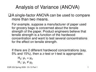
Chapter 19 Analysis of Variance (ANOVA). ANOVA. How to test a null hypothesis that the means of more than two populations are equal. H 0 : m 1 = m 2 = m 3 H 1 : Not all three populations are equal Test hypothesis with ANOVA procedure (Analysis of variance)

Chapter 19 Analysis of Variance (ANOVA)
E N D
Presentation Transcript
ANOVA • How to test a null hypothesis that the means of more than two populations are equal. H0: m1 = m2 = m3 H1: Not all three populations are equal • Test hypothesis with ANOVA procedure (Analysis of variance) • ANOVA tests use the F distribution
F Distribution • F distribution has 2 numbers of degree of freedom (DF) -- numerator and denominator. • EXAMPLE: df = (8,14) • Change in numerator df has a greater effect on the shape of the distribution. • Properties: • Continuous and skewed to the right • Has 2 df numbers • Nonnegative unites.
Finding the F valueExample 19.1 SITUATION: Find the F value for 8 degrees of freedom for the numerator, 14 degrees of freedom for the denominator and .05 area in the right tail of the F curve. • Consult Table V of Appendix A • corresponding to .05 area. • Locate the numerator on the top row, and the denominator along the left. • Find where they intersect. • This will give the critical value of F. • Excel: FDIST (x, df1, df2), FINV(prob., df1, df2)
Assumptions in ANOVA To test H0: m1=m2=m3 H1: Not all three populations are equal • The following must be true: • Population from which samples are drawn are normally distributed • Population from which the samples are drawn have the same variance (or standard deviation) • The samples are drawn from different populations that are random and independent.
How does ANOVA work? • The purpose of ANOVA is to test differences in means (for groups or variables) for statistical significance. • By partitioning the total variance into the component that is due to true random error (i.e., within-group SSE) and the components that are due to differences between groups (SSG). • SSG is then tested for statistical significance, and, if significant, the null hypothesis of no differences between means is rejected. • Always right-tailed with the rejection region in the right tail
Types of ANOVA • One-way ANOVA: Only one factor is considered • Two-way ANOVA • Answer the question if the tow categorical variables act together to impact the averages for the various groups? • If the two factors do not act together to impact the averages, does at least one of the factors have an impact on the averages for the various groups? • N-way ANOVA • Looking for interaction of multiple factors. • Requires more data • Always right-tailed with the rejection region in the right tail
ANOVA Notation and Formulas • xi = sample mean for group (or treatment) i • k = the number of groups (or treatments) • ni = sample size of group i • x = the average (the grand mean) of all of the observations in all groups • n = sum of the k sample sizes = n1 + n2 + n3 …. + nk • si2 = the sample variance for group (or treatment) i
MSG and MSE • Sum of squares for groups (SSG) • Mean squares for groups (MSG) • Sum of squared error (SSE) • Mean squared error (MSE)
SST and relationship among the SSs • Total sum of squares (SST) • SST is the numerator when calculating sample variance • Does not include a group distinction • Dividing SST by its df sample variance • Relationships SSG + SSE = SST
ANOVA Tables • It is common practice to report results using an ANOVA table:
ANOVA process by handExample 19.2 SITUATION: Soap manufacturer wants to test 3 new machines that should fill a jug. They tested for 5 hours and recorded the number of jugs filled by each per hour: • At the 10% significance level can we reject the null hypothesis that the mean number of jugs filled per hour by each machine is the same? • k = 3 • n1= n2 =n3 = 5 continued….
ANOVA process by handExample 19.2 continued • We now need to calculate the ANOVA table • For machine 1: • Now do the same for machine 2 & 3 • Then for 1-3 combined
ANOVA process by handExample 19.2 continued • Then we can calculate SSG/E/T: SST =SSG + SSE = 58.5335 + 111.2 = 169.7335 • Degrees of freedom • Group df = k-1 = 3-1 = 2 • Error df = n-k = 15-3 = 12 • Total df = n-1 = 15-1 = 14 continued….
ANOVA process by handExample 19.2 continued • Now calculate MSG, MSE, and F • Determine if the assumption that the three populations have the same population variance are valid. The assumption is reasonable if: • Now, look in Table V of Appendix A . Use numerator df=2, denominator df=12 …. continued….
Example 19.2 ANOVA tables • Replace the calculations results in the table below: • Do we reject the null hypothesis? H0: m1=m2=m3 H1: Not all three populations are equal
Example 19.2 by Minitab One-way ANOVA: P versus M Source DF SS MS F P M 2 58.53 29.27 3.16 0.079 Error 12 111.20 9.27 Total 14 169.73 S = 3.044 R-Sq = 34.49% R-Sq(adj) = 23.57% Individual 95% CIs For Mean Based on Pooled StDev Level N Mean StDev -+---------+---------+---------+-------- M1 5 51.600 3.050 (---------*---------) M2 5 55.200 3.194 (---------*---------) M3 5 50.600 2.881 (---------*---------) -+---------+---------+---------+-------- 48.0 51.0 54.0 57.0 Pooled StDev = 3.044
Example 19.3 by Minitab One-way ANOVA: Cus. versus Teller Source DF SS MS F P Teller 3 255.6 85.2 8.42 0.001 Error 18 182.2 10.1 Total 21 437.8 S = 3.182 R-Sq = 58.38% R-Sq(adj) = 51.45% Individual 95% CIs For Mean Based on Pooled StDev Level N Mean StDev ------+---------+---------+---------+--- A 5 21.600 3.362 (--------*-------) B 6 14.500 2.739 (------*-------) C 6 15.500 3.619 (-------*-------) D 5 22.000 2.915 (--------*-------) ------+---------+---------+---------+--- 14.0 17.5 21.0 24.5 Pooled StDev = 3.182
Pairwise Comparisons • If the result of ANOVA is to reject the null hypothesis, it does not identify which group means are significantly different. • Most software packages include this comparison. • Calculate a confidence interval for the differences of each unique pair of means. • Check to see if ZERO falls in the interval, if not then they are significantly different.
Example 19.3 by Minitab Fisher 95% Individual Confidence Intervals All Pairwise Comparisons Simultaneous confidence level = 80.96% A subtracted from: Lower Center Upper ---------+---------+---------+---------+ B -11.147 -7.100 -3.053 (------*------) C -10.147 -6.100 -2.053 (------*------) D -3.827 0.400 4.627 (------*------) ---------+---------+---------+---------+ -6.0 0.0 6.0 12.0 B subtracted from: Lower Center Upper ---------+---------+---------+---------+ C -2.859 1.000 4.859 (------*-----) D 3.453 7.500 11.547 (------*-----) ---------+---------+---------+---------+ -6.0 0.0 6.0 12.0 C subtracted from: Lower Center Upper ---------+---------+---------+---------+ D 2.453 6.500 10.547 (------*------) ---------+---------+---------+---------+ -6.0 0.0 6.0 12.0
Pairwise ComparisonsFisher’s Least Significant Difference (LSD) Method • Null Hypothesis: H0: i = j • Least Significant Difference (LSD) : • The pair of means iand j is declared significantly different if
Welch’s Approach to Heterogeneity of Variance • If Max(sj2)/Min(sj2)>2, the assumption of equal variance can not be used. • Welch’s approach modifies the F-test with the following steps: • For each sample j, calculate wj • Calculate the summation of w from k samples • Calculate the weighted avg. of sample means • Calculate the test statistic F0 and df