Computational Problems in Genetic Linkage Analysis: Insights and Case Studies
370 likes | 479 Vues
This talk explores the computational challenges in genetic linkage analysis, highlighted through collaboration with Ma'ayan Fishelson from Technion. Attendees will learn about the fundamental concepts of genetics, including chromosomes, markers, loci, and alleles, and their implications in identifying disease-causing genes. A case study on Werner's Syndrome illustrates practical applications, while relevant mathematics and software algorithms for gene hunting are discussed. Participants are expected to engage with course requirements, including a homework assignment and potential project continuation.

Computational Problems in Genetic Linkage Analysis: Insights and Case Studies
E N D
Presentation Transcript
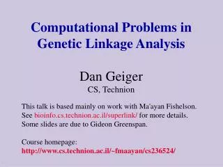
Computational Problems in Genetic Linkage Analysis Dan Geiger CS, Technion This talk is based mainly on work with Ma'ayan Fishelson. See bioinfo.cs.technion.ac.il/superlink/ for more details. Some slides are due to Gideon Greenspan. Course homepage: http://www.cs.technion.ac.il/~fmaayan/cs236524/ .
Requirements • One homework assignment (10%). • Mid term progress report. • Submission in pairs. • Well documented, tested, useful program. • Self initiative (by reading and thinking) will be rewarded. • One or two excelling projects maybe selected for continuation next semester under special projects course, if desired.
Part I: Quick look on relevant geneticsPart II: Case study: Werner’s syndrome Part III: Relevant Mathematics Part IV: Software description / algorithms Gene Hunting: find genes responsible for a given diseaseMain idea: If a disease is statistically linked with a marker on a chromosome, then tentatively infer that a gene causing the disease is located near that marker. Outline
Human Genome Most human cells contain 46 chromosomes: • 2 sex chromosomes (X,Y): XY – in males. XX – in females. • 22 pairs of chromosomes named autosomes.
Chromosome Logical Structure Marker – Genes, Single Nucleotide Polymorphisms, Tandem repeats, etc. Locus – the location of markers on the chromosome. Allele – one variant form (or state) of a gene/marker at a particular locus. Locus1 Possible Alleles: A1,A2 Locus2 Possible Alleles: B1,B2,B3
Alleles • b- dominant allele. Namely, (b,b), (b,w) is Black. • w - recessive allele. Namely, only (w,w) is White. This is an example of an X-linked trait. For males b alone is Black and w alone is white. genotype phenotype
Genotypes versus Phenotypes • At each locus (except for sex chromosomes) there are 2 genes. These constitute the individual’s genotype at the locus. • The expression of a genotype is termed a phenotype. For example, hair color, weight, or the presence or absence of a disease.
Recombination Phenomenon Male or female A recombination between 2 genes occurred if the haplotype of the individual contains 2 alleles that resided in different haplotypes in the individual's parent. (Haplotype – the alleles at different loci that are received by an individual from one parent). תאי מין: ביצית, או זרע
An example - the ABO locus. • The ABO locus determines detectable antigens on the surface of red blood cells. • The 3 major alleles (A,B,O) interact to determine the various ABO blood types. • O is recessive to A and B. Alleles A and B are codominant. Note: genotypes are unordered.
O A2/A2 A A1/A1 1 2 A A2/A2 A A1/A2 3 4 A | O A2 | A2 A O A1 A2 O O A2 A2 O O A1 A2 Recombinant O A1/A2 5 Example: ABO, AK1 on Chromosome 9 Phase inferred Male recombination fraction 12/100 and female 20/100. These numbers are measured in centi-morgans. One centi-morgan means one recombination every 100 meiosis. Ten centi-morgan corresponds to approx 1M nucleotides (with large variance) depending on the location and sex.
D A2/A2 H A1/A1 1 2 H A2/A2 H A1/A2 3 4 H | D A2 | A2 H D A1 A2 D D A2 A2 D D A1 A2 Recombinant D A1/A2 5 Example for Finding Disease Genes Phase inferred We use a marker with codominant alleles A1/A2. We speculate a locus with alleles H (Healthy) / D (affected) If the expected number of recombinants is low (close to zero), then the speculated locus and the marker are tentatively physically closed.
H A2/A2 H A1/A1 Phase ??? 1 2 H A2/A2 H A1/A2 3 4 Possible Recombinant D D A1 A2 H D A1 A2 H | D A2 | A2 D A1/A2 5 Recombination cannot be simply counted One can compute the probability that a recombination occurred and use this number as if this is the real count.
Comments about the example Often: • Pedigrees are larger and more complex. • Not every individual is typed. • Recombinants cannot always be determined. • There are more markers and they are polymorphic (have more than two alleles).
Genetic Linkage Analysis • The method just described is called genetic linkage analysis. It uses the phenomena of recombination in families of affected individuals to locate the vicinity of a disease gene. • Recombination fraction is measured in centi morgans and can change between males and females. • Next step: Once a suspected area is found, further studies check the 20-50 candidate genes in that area.
Part II: Case study Werner’s Syndrome A successful application of genetic linkage analysis
The Disease • First references in 1960s • Causes premature ageing • Autosomal recessive • Linkage studies from 1992 • WRN gene cloned in 1996 • Subsequent discovery of mechanisms involved in wild-type and mutant proteins
One Pedigree’s Data (out of 14) Pedigree number Father’s ID Sex: 1=male 2=female Unknown marker alleles 1 115 0 0 2 1 0 1 0 1 2 1 2 3 3 1 2 1 1 1 3 2 2 1 0 0 1 0 1 0 1 0 1 126 0 0 1 1 0 0 1 0 1 2 1 2 3 3 1 2 1 1 1 3 2 2 1 0 0 1 0 1 1 0 1 111 0 0 1 1 0 1 0 1 2 0 2 0 3 1 2 1 1 1 3 1 2 1 0 0 1 0 1 0 0 0 1 122 111 115 2 1 0 0 0 0 0 0 0 0 0 0 0 0 0 0 0 0 0 0 0 0 0 0 0 0 0 0 1 125 0 0 2 1 0 0 0 0 0 0 0 0 0 0 0 0 0 0 0 0 0 0 0 0 0 0 0 0 0 0 1 121 111 115 1 1 2 0 1 2 1 2 3 3 1 2 1 1 1 3 2 2 1 0 0 1 0 1 0 1 0 1 1 135 126 122 2 1 0 0 0 0 0 0 0 0 0 0 0 0 0 0 0 0 0 0 0 0 0 0 0 0 0 0 1 131 121 125 1 1 0 0 0 0 0 0 0 0 0 0 0 0 0 0 0 0 0 0 0 0 0 0 0 0 0 0 1 141 131 135 2 2 1 2 1 1 1 1 1 1 1 1 1 1 1 1 1 1 1 1 1 1 1 1 1 1 1 1 Known marker alleles Individual ID Mother’s ID Status: 1=healthy 2=diseased
Marker File Input 1 disease locus + 13 markers 14 0 0 5 0 0.0 0.0 0 1 2 3 4 5 6 7 8 9 10 11 12 13 14 1 2 0.995 0.005 1 0 0 1 3 6# D8S133 0.0200 0.3700 0.4050 0.0050 0.0500 0.0750 ...[other 12 markers skipped]... 0 0 10 7.6 7.4 0.9 6.7 1.6 2.5 2.8 2.1 2.8 11.4 1 43.8 1 0.1 0.45 Recessive disease requires 2 mutant genes First marker has 6 alleles First marker’s name Recombination distances between markers First marker founder allele frequencies
Genehunter Output position LOD_score information 0.00 -1.254417 0.224384 1.52 2.836135 0.226379 ...[other data skipped]... 18.58 13.688599 0.384088 19.92 14.238474 0.401992 21.26 14.718037 0.426818 22.60 15.159389 0.462284 22.92 15.056713 0.462510 23.24 14.928614 0.463208 23.56 14.754848 0.464387 ...[other data skipped]... 81.84 1.939215 0.059748 90.60 -11.930449 0.087869 Putative distance of disease gene from first marker in recombination units Log likelihood of placing disease gene at distance, relative to it being unlinked. Most ‘likely’ position Maximum log likelihood score
Final Location Marker D8S259 location of marker D8S339 Marker D8S131 WRN Gene final location Error in location by genetic linkage of about 1.25M base pairs.
The Maximum Likelihood Approach The probability of pedigree data Pr(data | ) is a function of the known and unknown recombination fractions denoted collectively by . How can we construct this likelihood function ? The maximum likelihood approach is to seek the value of which maximizes the likelihood function Pr(data | ) . This value is called the ML estimate. The main computational difficulty is to compute Pr(data|) for a specific value of .
Constructing the Likelihood function First, we need to determine the variables that describe the problem. There are several possible choices. Some variables we can observe and some we cannot. Lijm (Lijf) = Maternal (paternal) allele at locus i of person j. The values of this variables are the possible alleles li at locus i. Xij= Unordered allele pair at locus i of person j. The values are pairs of ith-locus alleles (li,l’i).
Constructing the Likelihood function L11f L11m Selector of maternal allele at locus 1 of person 3 X11 S13m P(s13m) = ½ L13m Maternal allele at locus 1 of person 3 (offspring) Selector variables Sijm are 0 or 1 depending on whose allele is transmitted to offspring i at maternal locus j. P(l13m | l11m, l11f,,S13m=0) = 1 if l13m = l11m P(l13m | l11m, l11f,,S13m=1) = 1 if l13m = l11f P(l13m | l11m, l11f,,s13m) = 0 otherwise
L11m L11f L12m L12f X11 S13m X12 S13f L13f L13m X13 L21m L21f L22m L22f X21 S23m X22 S23f L23f L23m X23 Model for locus 2 Probabilistic model for two loci Model for locus 1
L21m L11m L21f L11f L12m L22m L12f L22f X21 X11 S13m S23m X12 X22 S13f S23f L13f L23f L13m L23m X23 X13 Probabilistic model for Recombination males females 2 is called the recombination fraction between loci 2 & 1.
The Data The data consists of an assignment to a subset of the variables {Xij}. In other words some (or all) persons are genotyped at some (or all) loci.
Probability of data (sum over all states of all hidden variables) Prob(data| 2) = P(x11 ,x12 ,x13 ,x21 ,x22 ,x23) = Prob(data| 2) = P(x11 ,x12 ,x13 ,x21 ,x22 ,x23) = l11m, l11f … s23f [P(l11m) P(l11f) P(x11 | l11m, l11f,) … P(s13m) P(s13f) P(s23m |s13m, 2) P(s23m |s13m, 2) ] Constructing the likelihood function P(l11m,l11f,x11,l12m,l12f,x12,l13m,l13f,x13, l21m,l21f,x21,l22m,l22f,x22,l23m,l23f,x23, s13m,s13f,s23m,s23f | 2) = Product over all local probability tables = P(l11m) P(l11f) P(x11 | l11m, l11f,) … P(s13m) P(s13f) P(s23m |s13m, 2) P(s23m |s13m, 2) The result is a function of the recombination fraction. The ML estimate is the 2 value that maximizes this function.
Modeling Phenotypes L11f L11m X11 S13m Y11 L13m Phenotype variables Yij are 0 or 1 depending on whether a phenotypic trait associated with locus i of person j is observed. E.g., sick versus healthy. For example model of perfect recessive disease yields the penetrance probabilities: P(y11 = sick | X11= (a,a)) = 1 P(y11 = sick | X11= (A,a)) = 0 P(y11 = sick | X11= (A,A)) = 0
Standard usage of linkage There are usually 5-15 markers. 20-30% of the persons in large pedigrees are genotyped (namely, their xij is measured). For each genotyped person about 90% of the loci are measured correctly. Recombination fraction between every two loci is known from previous studies (available genetic maps). The user adds a locus called the “disease locus” and places it between two markers i and i+1. The recombination fraction ’between the disease locus and marker i and ” between the disease locus and marker i+1 are the unknown parameters being estimated using the likelihood function. This computation is done for every gap between the given markers on the map. The MLE hints on the whereabouts of a single gene causing the disease (if a single one exists).
Part IV: Software and Algorithms • Fastlink v4.1 (Each person’s genotype is one variable) • Vitesse v1,v2 (Only loopless Bayesian networks allowed) • GeneHunter/Alegro (exponential in number of persons) • Many more specific packages (e.g., affected siblings) • Superlink: Why is it better ? For a list, See http://linkage.rockefeller.edu/soft/list.html
SUPERLINK • Stage 1: each pedigree is translated into a Bayesian network. • Stage 2: value elimination is performed on each pedigree (i.e., some of the impossible values of the variables of the network are eliminated). • Stage 3: an elimination order for the variables is determined, according to some heuristic. • Stage 4: the likelihood of the pedigrees given the values is calculated using variable elimination according to the elimination order determined in stage 3.
over 100 hours Out-of-memory Pedigree size Too big for Genehunter. Experiment A • Same topology (57 people, no loops) • Increasing number of loci (each one with 4-5 alleles) • Run time is in seconds.
Bus error Out-of-memory Experiment C • Same topology (5 people, no loops) • Increasing number of loci (each one with 3-6 alleles) • Run time is in seconds.
Example: Matrix multiplication: versus Multidimensional multiplication/summation: The computational task at hand
Some options for improving efficiency • Performing approximate calculations of the likelihood. • Multiplying special probability matrices efficiently. • Grouping alleles together and removing inconsistent alleles. • Optimizing the elimination order of variables in a Bayesian network.
Project No. Project Subject 1 Performing approximate likelihood computations by using the method Iterative Join-Graph Propagation. (ps) 2 Performing haplotyping on the input data, i.e., inferring the most likely haplotypes for the individuals in the input pedigrees. (ps) 3 Performing approximate likelihood computations by using a heuristic which ignores extreme markers in the likelihood computation. (ps) Projects