Download
1 / 30
380 likes | 778 Vues
How do Radio Telescopes work?. K. Y. Lo. Electromagnetic Radiation. Wavelength. Radio Detection techniques developed from meter-wave to submillimeter-wave: = 1 meter = 300 MHz = 1 mm = 300 GHz. General Antenna Types Wavelength > 1 m (approx) Wire Antennas

E N D
How do Radio Telescopes work? K. Y. Lo
Electromagnetic Radiation Wavelength Radio Detection techniques developed from meter-wave to submillimeter-wave: = 1 meter = 300 MHz = 1 mm = 300 GHz
General Antenna Types Wavelength > 1 m (approx) Wire Antennas Dipole Yagi Helix or arrays of these Wavelength < 1 m (approx) Reflector antennas Wavelength = 1 m (approx) Hybrid antennas (wire reflectors or feeds) Feed
REFLECTOR TYPES Prime focus Cassegrain focus (GMRT) (AT) Offset Cassegrain Naysmith (VLA) (OVRO) Beam Waveguide Dual Offset (NRO) (ATA)
REFLECTOR TYPES Prime focus Cassegrain focus (GMRT) (AT) Offset Cassegrain Naysmith (VLA) (OVRO) Beam Waveguide Dual Offset (NRO) (ATA)
What do Radio Astronomers measure? • Luminosity of a source: L = dE/dt erg/s • Flux of a source at distance R: S = L/4R2 erg/s/cm2 • Flux measures how bright a star is. In optical astronomy, this is measured in magnitudes, a logarithmic measure of flux. • Intensity: If a source is extended, its surface brightness varies across its extent. The surface brightness is the intensity, the amount of flux that originates from unit solid angle of the source: I = dS/d erg/s/cm2/steradian
Measures of Radiation • The following should be clear: L = S d = 4R2 S for isotropic source 4 S = I d source • Since astronomical sources emit a wide spectrum of radiation, L, S and I are all functions of or , and we need to be more precise and define: • Luminosity density: L() = dL/d W/Hz • Flux density: S() = dS/d W/m2/Hz • Specific intensity: I() = dI/d W/m2/str/Hz • The specific intensity is the fundamental quantity characterizing radiation. It is a function of frequency, direction, s, and time. • In general, the energy crossing a unit area oriented at an angle to s, specified by the vector da, is given by dE = I(, s, t) sda d d dt = I(, ) sda d d dt
Analogs in optical astronomy • Luminosity is given by absolute magnitude • Flux, or brightness, is given by magnitudes within defined bands: U, B, V • Intensity, or surface brightness, is given by magnitude per square arc-second • Optical measures are logarithmic because the eye is roughly logarithmic in its perception of brightness • Quantitatively, a picture is really an intensity distribution map
Rayleigh-Jeans Law and Brightness Temperature • The Specific Intensity of thermal radiation from a black-body at temperature T is given by the Planck Distribution: I = (2h3/c2)/[exp(h/kT) 1] = (2hc3/2)/[exp(hc/kT) 1] = 2kT/2 if >> hc/kT or h << kT, R-J Law • Brightness Temperature Tb (2/2k) I = T for thermal radiation • Brightness temperature of the Earth at 100 MHz ~ 108 K (due to TV stations)
Antenna = Radio Telescope • The function of the antenna is to collect radio waves, and each antenna presents a cross section, or Effective Area, Ae(, ), which depends on direction (, ) • The power collected per unit frequency by the antenna from within a solid angle d about the direction (, ) is given by dP = ½ I(, ) Ae(, ) d W/Hz The ½ is because the typical radio receiver detects only one polarization of the radiation which we assume to be unpolarized.
The power density collected by the antenna from all directions is P = ½ I(, ) Ae(, ) d W/Hz • Antenna Temperature TA is defined by TA = P/k in K (Nyquist Theorem) • Therefore TA= (1/2k) I(, ) Ae(, ) d K • For a point source, I = S (, ) kTA= ½ Ae,max S W/Hz if Ae(, ) has a maximum value Ae,max at (, ) = (0, 0) • (Maximum) Effective Area of an antenna: Ae,max = ap Ag m2 where Ag is the geometric area and ap is the aperture efficiency. But, for a dipole antenna, Ag is zero but Ae is not.
Antenna pattern: Pn(,) = Ae(,)/Ae,max Pn(0,0) = 1 if the pattern is maximum in the forward direction • If the antenna is pointed at direction (o,o) TA (o,o)= (1/2k) I(, ) Ae(o, o) d In terms of Tb and Pn , TA (o,o)= (Ae,max/2) Tb(, ) Pn(o, o) d = (1/A) Tb(, ) Pn(o, o) d where 2/Ae,max= A. Note the antenna temperature, which measures the power density P (W/Hz) collected by the antenna is the convolution of the antenna pattern Pn with the source brightness distribution Tb
Antenna Properties Effective area: Ae(,,) m2 On-axis response Ae,max = Ag = aperture efficiency Normalized power pattern (primary beam) Pn(,,) = Ae(,,)/Ae,max Beam solid angle A= Pn(,,) d 4, = frequency all sky = wavelength Ae,max A = 2
Mapping by an Antenna TA (o,o)= (Ae,max/2) Tb(, ) Pn(o, o) d • Point source: Tb(, ) = (2/2k)S (, ) TA (o,o)= (Ae,max/2) (2/2k)S (, ) Pn(o, o) d = (Ae,max/2k) SPn(o, o) • Antenna pattern can be determined by scanning a point source • If pointing at the point source, then kTA = ½ Ae,maxS • If S is known, then Ae,max can be determined by measuring TA • Unresolved source: s < m ~ A 2/Ae,max TA (0, 0)= (Ae,max/2) Tb(, ) Pn(, ) d = (s/ A) Tb = (m/ A) (s/ m) Tb TA= m(s/ m) Tb Beam dilution
Maxwell Equations? • Radio telescopes operate in the physical optics regime, ~ D, instead of the geometric optics regime, << D, of optical telescope diffraction of radiation important • Easier to think of a radio telescope in terms of transmitting radiation • A point source of radiation (transmitter) at the focus of a paraboloid is designed to illuminate the aperture with a uniform electric field • The diffraction of the electric field across the aperture according to Huygens’ Principle determines the propagation of the electric field outward from the aperture or primary telescope surface • The transmitted electric field at a distant (far-field) point P in the direction (,) is given by the Fourier Transform of the electric field distribution across the aperture u(, ): u(,) u(, ) exp[2( + )/] dd
Antenna Pattern: Directional Response • Field Pattern of an antenna is defined by the Fourier Transform of the illumination of the aperture: u(,) u(, ) • Antenna Pattern is defined in terms of power or the square of the E field,|u|2. Pn(,) = |u(,)|2/|u(0,0)|2 • Alternately, the antenna pattern is proportional to the Fourier Transform of the auto-correlation function of the aperture illumination, u(, )
|u ()|2 Aperture-Beam Fourier Transform Relationship u (, ) = aperture illumination = Electric field distribution across the aperture (, ) = aperture coordinates ; u(,) = far-field electric field ( , ) = direction relative to “optical axis” of telescope : : |u ()|2
Types of Antenna Mount + Beam does not rotate + Lower cost + Better tracking accuracy + Better gravity performance - Higher cost - Beam rotates on the sky - Poorer gravity performance - Non-intersecting axis
Subreflector mount Reflector structure Antenna pointing design Quadrupod El encoder Alidade structure Rail flatness Foundation Az encoder
What happens to the signal collected by the antenna? Heterodyne Detection • At the focus, the radiation is collected by the receiver through a “feed” into a receiver that “pre-amplifies” the signal. • Then, the signal is mixed with a local oscillator signal close in frequency to the observing frequency in a nonlinear device (mixer). • The beat signal (IF or intermediate frequency signal) is usually amplified again before going through a bandwidth defining filter. (Frequency translation) • Then the IF signal is detected by a • square-law detector. RF at fsky Pre-amplifier LO at fLO IF at fsky fLO Amplification and filtering Voltage |E|2
VLA VLA and EVLA Feed System Design EVLA
Receivers in the telescope PF 1-1: 0.29 - 0.40 GHz PF 1-2: 0.38 - 0.52 PF 1-3: 0.51 - 0.69 PF 1-4: 0.68 - 0.92 PF 2 : 0.91 - 1.23 L : 1.15 - 1.73 GHz S : 1.73 - 2.60 C : 3.95 - 5.85 X : 8.00 - 10.0 Ku : 12.0 - 15.4 K1 : 18.0 - 22.0 K2 : 22.0 - 26.5 Q : 40.0 - 52.0 Gregorian Receiver Room
Radiometer Equation • For an unresolved source, the detection sensitivity of a radio telescope is determined by the effective area of the telescope and the “noisiness” of the receiver • For an unresolved source of a given flux, S, the expected antenna temperature is given by kTA = ½ Ae,maxS • The minimum detectable TA is given by TA = Ts/(B) where Ts is the system temperature of the receiver, B is the bandwidth and is the integration time, and is of order unity depending on the details of the system. The system temperature measures the noise power of the receiver (Ps = BkTs). In Radio Astronomy,detection is typically receiver noise dominated.
High Resolution: Interferometry Resolution /D 5 cm/100m = 2 arc-minute Uses smaller telescopes to make much larger 'virtual' telescope Maximum distance between antennas determines resolution VLA = 22-mile diameter radio telescope 5 cm/22 miles = 0.3 arc-second Aperture Synthesis: Nobel Prize 1974 (Ryle) D
VLA = Very Large Array (1980)Plain of San Augustine, New Mexico 27-antenna array: Extremely versatile Most productive telescope on ground
Interacting Galaxies • Optical image (left) shows nothing of the Hydrogen gas revealed by radio image by VLA (right).
Very Long Baseline Array • 10 25m antennas • Continent-wide: 5400-mile diameter radio telescope • 6 cm/5400 miles = 0.001 arc-second • Highest resolution imaging telescope in astronomy: 1 milli-arc-second = reading a news-paper at a distance of 2000 km