Download
1 / 24
250 likes | 512 Vues
KSU Math Department Colloquium. Graphical Models of Probability for Causal Reasoning. Thursday 07 November 2002 (revised 09 December 2003) William H. Hsu Laboratory for Knowledge Discovery in Databases Department of Computing and Information Sciences Kansas State University

E N D
KSU Math Department Colloquium Graphical Models of Probabilityfor Causal Reasoning Thursday 07 November 2002 (revised 09 December 2003) William H. Hsu Laboratory for Knowledge Discovery in Databases Department of Computing and Information Sciences Kansas State University http://www.kddresearch.org This presentation is: http://www.kddresearch.org/KSU/CIS/BN-Math-20021107.ppt
Overview • Graphical Models of Probability • Markov graphs • Bayesian (belief) networks • Causal semantics • Direction-dependent separation (d-separation) property • Learning and Reasoning: Problems, Algorithms • Inference: exact and approximate • Junction tree – Lauritzen and Spiegelhalter (1988) • (Bounded) loop cutset conditioning – Horvitz and Cooper (1989) • Variable elimination – Dechter (1996) • Structure learning • K2 algorithm – Cooper and Herskovits (1992) • Variable ordering problem – Larannaga (1996), Hsu et al. (2002) • Probabilistic Reasoning in Machine Learning, Data Mining • Current Research and Open Problems
Stages of Data Mining andKnowledge Discovery in Databases Adapted from Fayyad, Piatetsky-Shapiro, and Smyth (1996)
Conditional Independence • X is conditionally independent (CI) from Y given Z (sometimes written X Y | Z) iff P(X | Y, Z) = P(X | Z) for all values of X,Y, and Z • Example: P(Thunder | Rain, Lightning) = P(Thunder | Lightning) T R | L • Bayesian (Belief) Network • Acyclic directed graph model B = (V, E, ) representing CI assertions over • Vertices (nodes) V: denote events (each a random variable) • Edges (arcs, links) E: denote conditional dependencies • Markov Condition for BBNs (Chain Rule): • Example BBN Exposure-To-Toxins Serum Calcium X6 X1 X3 Age Cancer X5 X2 X4 X7 Gender Smoking Lung Tumor Graphical Models Overview [1]:Bayesian Networks P(20s, Female, Low,Non-Smoker, No-Cancer,Negative,Negative) = P(T) · P(F)·P(L | T) · P(N | T,F) · P(N | L, N) · P(N | N) · P(N | N)
X E Y Z (1) Z (2) Z (3) Graphical Models Overview [2]:Markov Blankets and d-Separation Property Motivation: The conditional independence status of nodes within a BBN might change as the availability of evidence E changes. Direction-dependent separation (d-separation) is a technique used to determine conditional independence of nodes as evidence changes. Definition: A set of evidence nodes Ed-separates two sets of nodes X and Y if every undirected path from a node in X to a node in Y is blocked given E. A path is blocked if one of three conditions holds: From S. Russell & P. Norvig (1995) Adapted from J. Schlabach (1996)
Graphical Models Overview [3]:Inference Problem Multiply-connected case: exact, approximate inference are #P-complete Adapted from slides by S. Russell, UC Berkeley http://aima.cs.berkeley.edu/
Other Topics in Graphical Models [1]:Temporal Probabilistic Reasoning • Goal: Estimate • Filtering: r = t • Intuition: infer current state from observations • Applications: signal identification • Variation: Viterbi algorithm • Prediction: r < t • Intuition: infer future state • Applications: prognostics • Smoothing: r > t • Intuition: infer past hidden state • Applications: signal enhancement • CF Tasks • Plan recognition by smoothing • Prediction cf. WebCANVAS – Cadez et al. (2000) Adapted from Murphy (2001), Guo (2002)
Other Topics in Graphical Models [2]:Learning Structure from Data • General-Case BBN Structure Learning: Use Inference to Compute Scores • Optimal Strategy: Bayesian Model Averaging • Assumption: models hH are mutually exclusive and exhaustive • Combine predictions of models in proportion to marginal likelihood • Compute conditional probability of hypothesis h given observed data D • i.e., compute expectation over unknown h for unseen cases • Let h structure, parameters CPTs Posterior Score Marginal Likelihood Prior over Parameters Prior over Structures Likelihood
Upward (child-to-parent) messages C4 C5 C1 C2 C3 C6 ’ (Ci’) modified during message-passing phase Downward messages P’ (Ci’) is computed during message-passing phase Propagation Algorithm in Singly-Connected Bayesian Networks – Pearl (1983) Multiply-connected case: exact, approximate inference are #P-complete (counting problem is #P-complete iff decision problem is NP-complete) Adapted from Neapolitan (1990), Guo (2000)
Find Maximal Cliques Triangulate A1 Clq4 Clq1 F6 B2 Moralize Clq2 G5 E3 B2 E3 G5 G C4 G A H F B A1 D8 B2 E3 D F6 H7 D B E A E F H C C G5 E3 Bayesian Network (Acyclic Digraph) C4 G5 Clq3 C4 C4 Clq6 C4 D8 Clq5 H7 Inference by Clustering [1]: Graph Operations (Moralization, Triangulation, Maximal Cliques) Adapted from Neapolitan (1990), Guo (2000)
Inference by Clustering [2]:Junction Tree – Lauritzen & Spiegelhalter (1988) • Input: list of cliques of triangulated, moralized graphGu • Output: • Tree of cliques • Separators nodes Si, • Residual nodes Ri and potential probability (Clqi) for all cliques • Algorithm: • 1. Si = Clqi(Clq1 Clq2 … Clqi-1) • 2. Ri = Clqi - Si • 3. If i >1 then identify a j < i such that Clqjis a parent of Clqi • 4. Assign each node v to a unique clique Clqi that v c(v) Clqi • 5. Compute (Clqi) = f(v) Clqi = P(v | c(v)) {1 if no v is assigned to Clqi} • 6. Store Clqi , Ri , Si, and (Clqi) at each vertex in the tree of cliques Adapted from Neapolitan (1990), Guo (2000)
Ri: residual nodes Si: separator nodes (Clqi): potential probability of Clique i AB (Clq1) = P(B|A)P(A) Clq1 = {A, B} A1 Clq1 Clq4 R1 = {A, B} Clq1 S1 = {} F6 B B2 BEC Clq2 (Clq2) = P(C|B,E) G5 E3 Clq2 = {B,E,C} Clq2 B2 E3 R2 = {C,E} S2 = { B } G5 EC E3 ECG Clq3 = {E,C,G} C4 Clq3 R3 = {G} (Clq3) = 1 G5 S3 = { E,C } Clq3 C4 EG CG C4 EGF (Clq4) = P(E|F)P(G|F)P(F) CGH (Clq5) = P(H|C,G) Clq6 C4 Clq5 Clq4 (Clq2) = P(D|C) D8 Clq4 = {E, G, F} Clq5 = {C, G,H} R4 = {F} R5 = {H} Clq5 C H7 S4 = { E,G } S5 = { C,G } CD Clq6 = {C, D} Clq6 R5 = {D} S5 = { C} Inference by Clustering [3]:Clique-Tree Operations Adapted from Neapolitan (1990), Guo (2000)
Age = [0, 10) X1,1 Age = [10, 20) X1,2 Age = [100, ) X1,10 Inference by Loop Cutset Conditioning • Deciding Optimal Cutset: NP-hard • Current Open Problems • Bounded cutset conditioning: ordering heuristics • Finding randomized algorithms for loop cutset optimization Split vertex in undirected cycle; condition upon each of its state values Exposure-To- Toxins Serum Calcium Number of network instantiations: Product of arity of nodes in minimal loop cutset Cancer X3 X6 X5 X4 X7 Smoking Lung Tumor X2 Gender Posterior: marginal conditioned upon cutset variable values
Inference by Variable Elimination [1]:Intuition Adapted from slides by S. Russell, UC Berkeley http://aima.cs.berkeley.edu/
Inference by Variable Elimination [2]:Factoring Operations Adapted from slides by S. Russell, UC Berkeley http://aima.cs.berkeley.edu/
Season A Rain Sprinkler B C F D Wet Manual Watering G Slippery Inference by Variable Elimination [3]:Example P(A), P(B|A), P(C|A), P(D|B,A), P(F|B,C), P(G|F) P(G|F) G=1 P(D|B,A) P(F|B,C) P(B|A) P(C|A) P(A) P(A|G=1) = ? d = < A, C, B, F, D, G > λG(f) = ΣG=1 P(G|F) Adapted from Dechter (1996), Joehanes (2002)
Genetic Wrapper for Change of Representation and Inductive Bias Control [2] Representation Evaluator for Learning Problems Dtrain(Inductive Learning) D: Training Data Dval(Inference) : Inference Specification f(α) Representation Fitness α Candidate Representation [1] Genetic Algorithm Optimized Representation Genetic Algorithms for Parameter Tuning in Bayesian Network Structure Learning
[A] Structure Learning G2 D: Data (User, Microarray) G = (V, E) G1 G4 G5 [B] Parameter Estimation G3 Treatment 1 (Control) Messenger RNA (mRNA) Extract 1 B = (V, E, ) cDNA Specification Fitness (Inferential Loss) Dval(Model Validation by Inference) G2 Treatment 2 (Pathogen) cDNA G1 G4 G5 DNA Hybridization Microarray (under LASER) Messenger RNA (mRNA) Extract 2 G3 Computational Genomics andMicroarray Gene Expression Modeling Learning Environment Adapted from Friedman et al. (2000) http://www.cs.huji.ac.il/labs/compbio/
Example Queries: • What experiments have found cell cycle-regulated metabolic pathways in Saccharomyces? • What codes and microarray data were used? How and why? Users of Scientific Workflow Repository Data Entity, Service, and Component Repository Index for Bioinformatics Experimental Research Learning over Workflow Instances and Use Cases (Historical User Requirements) Use Case & Query/Evaluation Data Personalized Interface User Queries & Evaluations Domain-Specific Collaborative Recommendation Decision Support Models Interface(s) to Distributed Repository Domain-Specific Workflow Repositories Workflows Transactional, Objective Views Workflow Components Data Sources, Transformations; Other Services DESCRIBER: An ExperimentalIntelligent Filter
Module 2 Learning & Validation of Relational Graphical Models (RGMs) for Experimental Workflows and Components Module 3 Estimation of RGM Parameters from Workflow and Component Database Structure & Data Training Data RGMs of Workflows Workflow Logs, Instances, Templates, Components (Services, Data Sources) Training Data Structure & Data Module 5 RGM Parameters from User Query Data Module 4 Learning & Validation of RGMs for User Requirements User Queries RGMs of Queries Personalized Interface Recommendations/Evaluations (Before and After Use) Module 1 Collaborative Recommendation Front-End Complete RGMsof User Queries CompleteRGMs of Workflows (Data-Oriented) Relational Graphical Modelsin DESCRIBER
Tools for Building Graphical Models • Commercial Tools: Ergo, Netica, TETRAD, Hugin • Bayes Net Toolbox (BNT) – Murphy (1997-present) • Distribution page http://http.cs.berkeley.edu/~murphyk/Bayes/bnt.html • Development group http://groups.yahoo.com/group/BayesNetToolbox • Bayesian Network tools in Java (BNJ) – Hsu et al. (1999-present) • Distribution page http://bndev.sourceforge.net • Development group http://groups.yahoo.com/group/bndev • Current (re)implementation projects for KSU KDD Lab • Continuous state: Minka (2002) – Hsu, Guo, Perry, Boddhireddy • Formats: XML BNIF (MSBN), Netica – Guo, Hsu • Space-efficient DBN inference – Joehanes • Bounded cutset conditioning – Chandak
References [1]:Graphical Models and Inference Algorithms • Graphical Models • Bayesian (Belief) Networks tutorial – Murphy (2001) http://www.cs.berkeley.edu/~murphyk/Bayes/bayes.html • Learning Bayesian Networks – Heckerman (1996, 1999) http://research.microsoft.com/~heckerman • Inference Algorithms • Junction Tree (Join Tree, L-S, Hugin): Lauritzen & Spiegelhalter (1988) http://citeseer.nj.nec.com/huang94inference.html • (Bounded) Loop Cutset Conditioning: Horvitz & Cooper (1989) http://citeseer.nj.nec.com/shachter94global.html • Variable Elimination (Bucket Elimination, ElimBel): Dechter (1986)http://citeseer.nj.nec.com/dechter96bucket.html • Recommended Books • Neapolitan (1990) – out of print; see Pearl (1988), Jensen (2001) • Castillo, Gutierrez, Hadi (1997) • Cowell, Dawid, Lauritzen, Spiegelhalter (1999) • Stochastic Approximation http://citeseer.nj.nec.com/cheng00aisbn.html
References [2]:Machine Learning, KDD, and Bioinformatics • Machine Learning, Data Mining, and Knowledge Discovery • K-State KDD Lab: literature survey and resource catalog (2002) http://www.kddresearch.org/Resources • Bayesian Network tools in Java (BNJ): Hsu, Guo, Joehanes, Perry, Thornton (2002) http://bndev.sourceforge.net • Machine Learning in Java (BNJ): Hsu, Louis, Plummer (2002) http://mldev.sourceforge.net • NCSA Data to Knowledge (D2K): Welge, Redman, Auvil, Tcheng, Hsu http://alg.ncsa.uiuc.edu • Bioinformatics • European Bioinformatics Institute Tutorial: Brazma et al. (2001) http://www.ebi.ac.uk/microarray/biology_intro.htm • Hebrew University: Friedman, Pe’er, et al. (1999, 2000, 2002) http://www.cs.huji.ac.il/labs/compbio/ • K-State BMI Group: literature survey and resource catalog (2002) http://www.kddresearch.org/Groups/Bioinformatics
Acknowledgements • Kansas State University Lab for Knowledge Discovery in Databases • Graduate research assistants: Haipeng Guo (hpguo@cis.ksu.edu), Roby Joehanes (robbyjo@cis.ksu.edu) • Other grad students: Prashanth Boddhireddy, Siddharth Chandak, Ben B. Perry, Rengakrishnan Subramanian • Undergraduate programmers: James W. Plummer, Julie A. Thornton • Joint Work with • KSU Bioinformatics and Medical Informatics (BMI) group: Sanjoy Das (EECE), Judith L. Roe (Biology), Stephen M. Welch (Agronomy) • KSU Microarray group: Scot Hulbert (Plant Pathology), J. Clare Nelson (Plant Pathology), Jan Leach (Plant Pathology) • Kansas Geological Survey, Kansas Biological Survey, KU EECS • Other Research Partners • NCSA Automated Learning Group (Michael Welge, Tom Redman, David Clutter, Lisa Gatzke) • The Institute for Genomic Research (John Quackenbush, Alex Saeed) • University of Manchester (Carole Goble, Robert Stevens) • International Rice Research Institute (Richard Bruskiewich)