Understanding Probability: Rules, Models, and Applications
Explore the fundamentals of probability, including randomness and chance. Learn about rules like the General Addition and Multiplication Rules, and how to apply them to different models like the Discrete and Continuous models. Understand the Normal Distribution and how it is utilized to analyze data. Dive into concepts like Conditional Probability and Independent Events, and see real-world examples of their application. Enhance your knowledge of probability with this comprehensive guide.

Understanding Probability: Rules, Models, and Applications
E N D
Presentation Transcript
Probability Definition: randomness, chance, likelihood, proportion, percentage, odds. Not sure what will happen in a single event but, in the long run, certain patterns emerge. Probability is the mathematical ideal. We use letters like X and Y to represent quantities. These will be called random variables.
Probability Model • List the outcomes for a given event (experiment or question) and associated probabilities. • S: sample space (contains all possible outcomes) • Event: single outcome or collection of outcomes • Example: pick a card out of a standard deck • S: sample space contains • Event: pick a • pick a
Basic Rules • Event A has probability P(A), which is between 0 and 1 (inclusive). • Probability of entire sample space, P(S), is . • Addition: If two events are disjoint (nothing in common), then P(A or B) = . • Complement: P(not A) =
Probability Model for standard deck of cards • 52 cards, 4 suits (Diamonds, Hearts, Clubs, Spades) • Each suit as 13 cards: 2, 3, 4, 5, … , 9, 10, J, Q, K, A • P(picking any single card)= • A = event that a red 5 is picked • B = event that a club is picked • C = event that a face card (J, Q, K) is picked • P(A or B)= • P(not C) =
Discrete Model • If sample space is finite, the probability model is called discrete. • List all outcomes and associated probabilities in a table. • Roll 2 six-sided dice and record the sum.
Continuous Model • If sample space contains a range of values, the probability model is called continuous. • Density curves record probabilityas the area under the • curve for a given range of outcomes. • So, total area under the curve will always equal 1.
Continuous Model – Example 1 • The uniform distribution for any real number, X, from 3 to 7 looks like: 3 5 7 3 5 6 7 3 5 7 5.1 3.2
Continuous Model – Example 2 • The symmetric triangular distribution for any real number, X, from 0 to 8 looks like: 4 8 4 8 4 8
More Probability Use Venn diagrams to visualize probability rules. Sample space, S: rectangle Events (A, B, C, …): circles inside If events are disjoint, don’t overlap circles. Keep track of # of outcomes in each region of the rectangle.
Venn diagram - example • Example: pick a card out of a standard deck • S: sample space contains 52 outcomes (52 cards) • A = event that a red 5 is picked • B = event that a club is picked • C = event that a face card (J, Q, K) is picked • S • B • A • C
P(A or B) • P(B or C) • S • S • B • B • 10 • 10 • A • A • 2 • 3 • 3 • 2 • 9 • 9 • 28 • 28 • C • C
General Addition Rule • A = event that a red card is picked • B = event that a number card is picked • P(A or B) • S • A • B • General Addition: P(A or B) =
Conditional Probability Rule • Given a condition (you know something happened), how • does that change the chances of something else happening? • P(B|A)= probability of B given A • S • A • B
Venn Diagram of 70 students • C: owns a cat • D: owns a dog • 10 • S • D • C • 30 • 20 • 10
General Multiplication Rule • Rewrite • to get: • Experiment: pick two cards out of a standard deck
Independent Events • Two (or more) events are independent if knowledge of one event does not change the chances of the other. • Multiplication Rule for Independent Events:
For a cholesterol-lowering drug, there is a 5% chance that a loss-of-sleep side effect will occur. • What are the chances that two people picked at random take the drug and experience sleep loss? • What are the chances that at least 1out of 3 loses sleep?
The Normal Distribution Use curves to describe overall pattern seen in a histogram. Curve will capture 100% of all observations. Hence, there will be a total area of 1 below it. Then the area under the curve for a given range of values will represent the proportion (percent, fraction) of observations that fall in that range.
Curves and proportions % • The proportion of scores above 80 is roughly 26.8%. v 40 60 20 80 100 % • The area under the density curve for scores above 80 is roughly 0.261 =26.1%. v 40 60 20 80 100
Mean and Medians • Location of the median on a density curve is where area under is cut in half. • Location of the mean on a density curve is where the length of the curve is cut in half. • On symmetric curves: • On skewed curves:
Normal curves are special kinds of density curves • Symmetric, single peaked, bell-shaped • Use m(mu) ands(sigma)to talk about mean and std. dev. • – • s – m m - s m + s
68-95-99.7 Rule • About 68% of data fall within • About 95% of data fall within • About 99.7% of data fall within m m + 2s m + 3s m - 3s m - 2s m - s m + s
Example 1 • Grasshopper jumps can be described by a Normal • distribution with m = 12 inches and s = 2 inches. • About 68% of all jumps are between inches. • About where would you find the top 2.5%? 68% 95% 99.7% 12 16 18 6 8 10 14
Example 1 – continued • What % falls below 14 inches? 12 12 16 18 16 18 8 6 6 8 10 14 10 14 16 18 6 8 10 14 12 • What % of jumps are more than 14 inches? • What % of jumps are between 14 and 16 inches?
Finding values without 68-95-99.7 • We use tables or calculators to find harder values, like where is the top 10% or what percent falls below a given observation. • N(m, s) means observations come from a Normal distribution with a mean of m and a standard deviation of s. • Standardize observationx from N(m, s) by: • The standardized value is called a
Two functions on the calculator • (found under 2nd VARS => DISTR) • normalcdf( : will give area between two bounds for a given m, s. • invNorm( : will give the observation that has a particular area to its left for a given m, s. • normalcdf(lower bound, upper bound, m, s) • invNorm(area, m, s) m m - s m + s
Using the calculator with grasshopper N(12, 2) • What % of jumps fall below 17 inches? • No lower bound, so: 12 16 18 8 6 10 14 • normalcdf(lower bound, upper bound, m, s) • = normalcdf( ) = area below 17 = • What % of jumps fall above 11.5 inches? • First, find area 12 16 18 8 6 10 14 • normalcdf(lower bound, upper bound, m, s) • = normalcdf( ) = area = • Since total area is 1 and we have : • we want
Using the table with grasshopper N(12, 2) • What % of jumps fall between 10 and 16.36 inches? • - • = 12 12 16 18 16 18 8 8 6 6 10 14 10 14 12 16 18 8 6 10 14 • Area between = area below 16.36 – area below 10. • Calculator does this all at once with the normalcdf( function. • normalcdf(lower bound, upper bound, m, s) • = normalcdf( ) = area between =
Using the table with grasshopper N(12, 2) • What jumps fell in the top 10%? • 10% 12 16 18 8 6 10 14 • What observation has an area of .10 above it? • What observation has an area of .90 below it? • Use invNorm function to find that observation. • invNorm(area, m, s) • = invNorm( ) = value with .9 area below=
Using the table with grasshopper N(12, 2) • 50% • Where do the middle 50% fall? 12 16 18 8 6 10 14 • What observation has an area of below it? • What observation has an area of below it? • Use invNorm function to find those observations. • invNorm(area, m, s) • = invNorm( ) = value with area below = • invNorm(area, m, s) • = invNorm( ) = value with area below =
68-95-99.7 Rule • 1,2,3 standard deviations away accurate to two decimal places
Sampling Distributions Know the entire population: (parameter) Know only a sample (SRS): (statistic)
Law of Large Numbers • - As you increase the sample size, sample mean gets closer to population mean • Population = 3, 3, 8, 15, 20, 21, 22, 31, 39 • Sample of size 1= 8 • Sample of size 2= 8, 22 • Sample of size 3= 8, 22, 31 • Sample of size 4= 8, 22, 31, 3 • Sample of size 5= 8, 22, 31, 3, 20
Population of 7 people and their weights (in pounds) • 122, 140, 150, 155, 160, 170, 195 • Samples of size 1: {122}, {140}, {150}, {155}, {160}, {170}, {195} • Mark off the sample mean for each sample with an “x” • x • x • x • x • x • x • x • 120 • 130 • 140 • 150 • 160 • 170 • 180 • 190 • 200 • Samples of size 2: {122, 140}, {122, 150}, {122, 155}, {122, 160}, {122, 170}, {122, 195}, {140, 150}, …, (170, 195}. There are 21 possible samples. • Mark off the sample mean for each sample with an “x” • x • x • x • x • x • x • x • x • x • x • x • x • x • x • x • x • x • x • x • x • x • 120 • 130 • 140 • 150 • 160 • 170 • 180 • 190 • 200
Population of 7 people (continued) • 140, 122, 160, 195, 150, 155, 170 • Samples of size 1: • x • x • x • x • x • x • x • 120 • 130 • 140 • 150 • 160 • 170 • 180 • 190 • 200 • Samples of size 2: • x • x • x • x • x • x • x • x • x • x • x • x • x • x • x • x • x • x • x • x • x • 130 • 140 • 150 • 160 • 170 • 180 • 190 • Samples of size 6: 7 possible sample of this size. {122, 140, 160, 150, 155, 170}, … • x • x • x • x • x • x • x • 140 • 150 • 160 • 170 • 180
Sampling distribution of • Sampling from a large population with mean m and • standard deviation s: • samples of size n will have their sample means distributed • with a mean m and standard deviation s over root n. • If population is N(m, s), then • If population is not Normal but n is large, then
Ex. 1 - Weight of eggs is N(65, 3) • Your egg carton holds 9 eggs, so consider each carton as a random sample of 9 eggs. Let X be the weight of a single egg in grams and X be average weight of your carton. • What is the sampling distribution for your carton’s average weight?
Weight of eggs is N(65, 3) – continuedMean weight of carton is N(65,1) • Convert 67 to a z-score • for the carton: • Convert 67 to a z-score • for a single egg: 67 56 59 68 71 62 65 74
Ex. 2 - Length of trout is N(17.5, 2.5) • Your local waters contain a multitude of trout. Let X be the length of a single fish in inchesandX be average length of your daily catch of five fish. • What is the sampling distribution for your daily catch?
Trout length is N(17.5, 2.5) – continuedMean length of daily catch is N(17.5,1.118) • Convert 16 to a z-score • for the daily catch: • Convert 16 to a z-score • for a single fish: 10 12.5 20 22.5 15 17.5 25
Trout length is N(17.5, 2.5) – continuedMean length of daily catch is N(17.5,1.118) 10 12.5 20 22.5 15 17.5 25 15 10 12.5 17.5 20 22.5 25
Ex 3 - Length of trout is N(10, 2) • Your fishing pond has another type of trout. Let X be the length of a single fish in inches taken at random andX be average length of a sample of 16 fish. • What is the sampling distribution for a sample of 16 fish?
Trout length is N(10, 2) – continuedMean length of 16 fish is N(10,0.5) 8 4 6 12 14 10 16 4 6 8 10 12 14 16

