Introduction to Adversarial Search in Artificial Intelligence

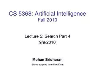
1. CS 5368: Artificial IntelligenceFall 2010 Lecture 5: Search Part 4 9/9/2010 Mohan Sridharan Slides adapted from Dan Klein

2. Announcements • Search assignment will be up shortly. • Notice change in assignment content and deadlines. • Include a few questions/comments in all future responses.

3. Today • Begin adversarial search!

4. Adversarial Search • Pacman adversarial by definition  • Agents have to contend with ghosts.

5. Game Playing • Many different kinds of games! • Axes: • Deterministic or stochastic? • One, two, or more players? • Perfect information (can you see the state)? • Need algorithms for computing a strategy (policy) which suggests a move in each state.

6. Deterministic Games • Many possible formalizations, one is: • States: S (start at s0) • Players: P={1...N} (usually take turns) • Actions: A (may depend on player / state) • Transition Function: SxA  S • Terminal Test: S  {t,f} • Terminal Utilities: SxP  R • Solution for a player is a policy: S  A

7. lose win lose Deterministic Single-Player? • Deterministic, single player, perfect information: • Know the rules and action results. • Know when you win. • Free-cell, 8-Puzzle, Rubik’s cube. • Just search! • Slight reinterpretation: • Each node stores a value: the best outcome it can reach. • This is the maximal outcome of its children. • No path sums (utilities at end). • After search, can pick move that leads to best node.

8. Deterministic Two-Player • Tic-tac-toe, chess, checkers. • Zero-sum games: • One player maximizes result. • The other minimizes result. • Chess! • Minimax search: • A state-space search tree. • Players take turns. • Each layer, or ply, consists of a round of moves*. • Choose move to position with highest minimax value = best achievable utility against best play. max min 8 2 5 6 * Slightly different from the book definition

9. Tic-tac-toe Game Tree

10. Minimax Example

11. Minimax Basics • Minimax(n) is the utility for MAX in being in that state, assuming both players play optimally from there to the end of the game! • Minimax of terminal state is the utility. • Simple recursive search computation and value backups (Figure 5.3).

12. Minimax Search

13. Minimax Properties • Optimal against a perfect player. Otherwise? • Time complexity? • O(bm) • Space complexity? • O(bm) • For chess, b  35, m  100 • Exact solution is completely infeasible. • Do we need to explore the whole tree? max min 10 10 9 100

14. Resource Limits • Cannot search to leaves! • Depth-limited search: • Search a limited depth of tree. • Replace utilities with an evaluation function for non-terminal positions. • Guarantee of optimal play is gone! • More plies makes a BIG difference  • Example: • Suppose we have 100 seconds, can explore 10K nodes / sec. • So can check 1M nodes per move. • - reaches about depth 8 – decent chess program. max 4 min min -2 4 -1 -2 4 9 ? ? ? ?

15. Evaluation Functions • Function which scores non-terminals. • Ideal function: returns the utility of the position. • In practice: typically weighted linear sum of features: • E.g. f1(s) = (num white queens – num black queens).

16. Evaluation for Pacman

17. Can Pacman Starve? • Knows score will go up by eating the dot now. • Knows score will go up just as much by eating the dot later on. • No point-scoring opportunities after eating the dot. • Therefore, waiting seems just as good as eating!

18. Iterative Deepening Iterative deepening uses DFS as a subroutine: • Do a DFS which only searches for paths of length 1 or less. (DFS gives up on any path of length 2). • If “1” failed, do a DFS which only searches paths of length 2 or less. • If “2” failed, do a DFS which only searches paths of length 3 or less. ….and so on. Do we want to do this for multiplayer games? b …

19. - Pruning • At node n: if player has better choice m at parent node of n or further up, n will never be reached!

20. - Pruning • General configuration: •  is the best value that MAX can get at any choice point along the current path. • If n becomes worse than , MAX will avoid it, so can stop considering n’s other children. • Define  similarly for MIN. • Figure 5.7 in textbook. Player Opponent  Player Opponent n

21.  v - Pruning Pseudocode

22. - Pruning Properties • Pruning has no effect on final result!  • Good move ordering improves effectiveness of pruning. (Section 5.3.1). • With “perfect ordering”: • Time complexity drops to O(bm/2) • Doubles solvable depth. • Full search of, e.g. chess, is still hopeless  • A simple example of meta-reasoning: reasoning about which computations are relevant.

23. Non-Zero-Sum Games • Similar to minimax: • Utilities are now tuples. • Each player maximizes their own entry at each node. • Propagate (or back up) nodes from children. 1,2,6 4,3,2 6,1,2 7,4,1 5,1,1 1,5,2 7,7,1 5,4,5

24. Advance Notice… • Get ready for: • Probabilities. • Expectations. • Upcoming topics (in a week): • Dealing with uncertainty. • How to learn evaluation functions. • Markov Decision Processes.