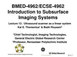
BMED-4962/ECSE-4962 Introduction to Subsurface Imaging Systems
BMED-4962/ECSE-4962 Introduction to Subsurface Imaging Systems. Lecture 12: Ultrasound scanner as a linear system Kai E. Thomenius 1 & Badri Roysam 2 1 Chief Technologist, Imaging Technologies, General Electric Global Research Center 2 Professor, Rensselaer Polytechnic Institute.

BMED-4962/ECSE-4962 Introduction to Subsurface Imaging Systems
E N D
Presentation Transcript
BMED-4962/ECSE-4962Introduction to Subsurface Imaging Systems Lecture 12: Ultrasound scanner as a linear system Kai E. Thomenius1 & Badri Roysam2 1Chief Technologist, Imaging Technologies, General Electric Global Research Center 2Professor, Rensselaer Polytechnic Institute Center for Sub-Surface Imaging & Sensing
THE BIG PICTURE What is subsurface sensing & imaging? Why a course on this topic? EXAMPLE: THROUGH TRANSMISSION SENSING X-Ray Imaging Computer Tomography COMMON FUNDAMENTALS propagation of waves interaction of waves with targets of interest PULSE ECHO METHODS Examples Multi-dimensional imaging MRI A different sensing modality from the others Basics of MRI MOLECULAR IMAGING What is it? PET & Radionuclide Imaging IMAGE PROCESSING & CAD Outline of Course Topics
Recap of Last Lecture • We have been introduced to the Field II simulation program and walked through some of the code. • We have used this Field II example to demonstrate the role of linear system theory in the understanding of imagers. • Our goal was to learn about ultrasound scanners as well as the tools we use to understand & design such systems.
Linear Systems • A linear system is completely characterized by its impulse response. • All the processing steps of an ultrasound scanner can be modeled as a set of impulse responses. • Luckily, all these steps have been incorporated in a software package called Field II
Ultrasound Scanner as a Linear System Propagation Path (1/2 of calc_hhp) Transmit Array (xdc_concave, Xdc_impulse) Pulser (excitation) Scattering Propagation Path (1/2 of calc_hhp) Receive Array (xdc_concave, Xdc_impulse) Display code • Each block in this system is covered by an impulse response or a transfer function. • As a consequence, the response of the entire system can be modeled as a convolution of the impulse responses or the product of the transfer functions.
Code Review • Last time we went through the “logo code” fairly quickly. • Let us finish the last two parts of the code with a bit more care.
From Last Class: Code Review • Call to xdc_concave: • Purpose: Procedure for creating a concave transducer • Calling: Th = xdc concave (radius, focal radius, ele size); • Input: • Radius: Radius of physical elements. • focal radius: Focal radius. • ele size: Size of mathematical elements. • Output: Th - A pointer to this transducer aperture. • Define transducer impulse response • Hanning-weighted sine wave • Define the transmit pulse • Excitation – sine wave • % Define the transducer • Th = xdc_concave (R, Rfocus, ele_size); • % Set the impulse response and excitation of the emit aperture • impulse_response=sin(2*pi*f0*(0:1/fs:2/f0)); • impulse_response=impulse_response.*hanning(max(size(impulse_response)))'; • xdc_impulse (Th, impulse_response); • excitation=sin(2*pi*f0*(0:1/fs:2/f0)); • xdc_excitation (Th, excitation); • % Calculate the pulse echo field and display it • xpoints=(-10:0.2:10); • [RF_data, start_time] = calc_hhp (Th, Th, [xpoints; zeros(1,101); 30*ones(1,101)]'/1000);
Code Review – PSF Determination • Call to calc_hhp: • Purpose: Procedure for calculating the pulse echo field. • Calling: [hhp, start time] = calc hhp(Th1, Th2, points); • Input: • Th1 Pointer to the transmit aperture. • Th2 Pointer to the receive aperture. • points Field points. Vector with three columns (x,y,z) and one row for each field point. • Output: • RF_data - Received voltage trace. • start time - The time for the first sample in RF_data. • % Calculate the pulse echo field and display it • xpoints=(-10:0.2:10); • [RF_data, start_time] = calc_hhp (Th, Th, [xpoints; zeros(1,101); 30*ones(1,101)]'/1000); • % Make a display of the envelope • figure(1) • env=abs(hilbert(RF_data(1:5:600,:))); • env=20*log10(env/max(max(env))); • [N,M]=size(env); • env=(env+60).*(env>-60) - 60; • mesh(xpoints, ((0:N-1)/fs + start_time)*1e6, env) • ylabel('Time [\mus]') • xlabel('Lateral distance [mm]') • title('Pulse-echo field from 8 mm concave transducer at 30 mm') • axis([-10 10 38.41 39.6 -60 0]) • view([-14 80])
Code Review – PSF Display • The highlighted lines perform the following steps to create the display: • hilbert is a matlab command which gives the envelope of an RF signal • 20*log10() converts the envelope to decibels • mesh is a matlab command for displaying 2D data • % Calculate the pulse echo field and display it • xpoints=(-10:0.2:10); • [RF_data, start_time] = calc_hhp (Th, Th, [xpoints; zeros(1,101); 30*ones(1,101)]'/1000); • % Make a display of the envelope • figure(1) • env=abs(hilbert(RF_data(1:5:600,:))); • env=20*log10(env/max(max(env))); • [N,M]=size(env); • env=(env+60).*(env>-60) - 60; • mesh(xpoints, ((0:N-1)/fs + start_time)*1e6, env) • ylabel('Time [\mus]') • xlabel('Lateral distance [mm]') • title('Pulse-echo field from 8 mm concave transducer at 30 mm') • axis([-10 10 38.41 39.6 -60 0]) • view([-14 80]) Field II is a very convenient tool that minimizes the work required to simulate any coherent scanner.
Goal of the Simulation – Point Spread Function for Transducer • We wish to determine the pulse-echo point spread function for this transducer. • What is that? • A point spread function (PSF) describes the response of an imaging system to a point source or point object. • A related but more general term for the PSF is a system's impulse response. • It can be used to characterize any imaging system. PSF of a confocal microscope – convolution with two targets and resulting image.
PSF from a Concave Source How would you get the point spread function of a CT scanner?
Optics – Airy Disc PSF http://www.optics.arizona.edu/jcwyant/Optics505(2000)/ChapterNotes/Chapter15/psfandmtfcurves.pdf
So, what is a tool like Field II good for? Here are a couple of examples …
Analysis of a complex transmit signal Regulatory Limits on Transmit Energy Determines Penetration Pulse Amplitude Mechanical Index Limit Pulse Length Longer pulse gains penetration but sacrifices resolution
Resolution / Penetration Dilemma 7 MHz 5 MHz Penetration limited due to Beer’s Law
1 1 1 0 1 0 1 1 Encoder Possible Solution: Coded Excitation Alternate encodings could use a chirp. Transmitted Pulse Train Body • Sensitivity Increase Received Pulse Train 1 1 0 1 0 1 1 1 Decoder Coded Excitation improves sensitivity without resolution tradeoff
The Matched Filter • Basic Idea: • Suppose you have a signal s(t) with a known shape corrupted by additive noise n(t). • We can construct a ‘matched filter’ m(t) that is designed to maximize our ability to detect s(t) • The matched filter is only a function of the transmitted signal’s shape (hence the name) • Its impulse response is a time reversed copy of s(t) with some scaling factor α that depends upon the noise * Indicates complex conjugate
Decoding • Decoding is done with matched or correlation filtering. • This is often implemented as a convolution. • Let us assume we transmit a code p(t) and receive signal s(t). • Matched filter can be implemented as the convolution of the received signal by the time-reversed transmit pulse. Hardware is readily available to implement convolution based filtering.
1 1 1 0 1 0 1 1 Encoder 1 1 0 1 0 1 1 1 Decoder How could we evaluate this with Field II? • Encoding step: • We need to define an excitation function to represent the coded signal. • This can be applied thru the xdc_excitation function. • Decoding step: • Implement the matched filter step in matlab. • Apply the resulting signal exactly the same way as any RF echo. • The rest of the processing is identical to any of the imaging examples given.
Coded Excitation - Experiment High Frequency Coded Excitation 15 cm 18 cm Improve penetration by 3 cm with same resolution to -50 dB
Utility of Tools like Field II • Here are some other applications: • Design tools • Evaluate an array design without building it. • Evaluate signal processing techniques • Use the phantoms to compare detectability of use defined lesions • Teach image formation techniques • Field II is the most commonly used design tool for medical ultrasound.
Current Ultrasound Battlefields • Another area which saw heavy use of Field II was 3D/4D ultrasound. • Next couple of slides show some of the key steps in getting there.
3D/4D Imaging • In CT, we learned about helical/spiral CT acquisition • This meant getting 3D data. • So what is 4D Imaging? • Time is the fourth dimension!
2D 3D 4D 3D imaging in real-time
Real-Time 3D 3D imaging: • Need to move acoustic beams in 3-space • Mechanical • Electronic • Multi-planar, real-time display: • longitudinal, transversal and horizontal planes • Volume or surface rendered 3D image sets • Volume rate (as opposed to the frame rate) becomes key 3D Voxel 2D Pixel
Mechanical 4D Solution Transducer Cable Drive Fluid-FilledHousing Stepper Motor Belt Drive Cable Optimized for high-speedmotion, up to 18 vol/sec
Mechanical Probe Images • Move a 1D array back and forth rapidly over a sector. • Volume rates in the order of 15 – 25 volumes/sec possible.
One Possible Solution • Migrate beamformer components to probe handle. • With multi-row probes, multiplexing is in the handle. • Patent by Larson from 1993 • group 2D array elements into subarrays • combine echoes from subarrays and send summed signals • cable count reduced w. reasonable spatial sampling. • Look for more system changes along these lines Probe Handle
Migration of Beamformation to Handle Modular Beamformerin Probe Handle 2D Transducer Array(vs. human hair)
Power &Control Preamps To SystemChannel Sum Delays Digital or Analog? Transmit Sub-Array Beamformer in Probe • Connects a group of transducer elements to each system channel • Low-power analog beamformer: Phase rotation or Delay lines • Small delays only: static steering of small sub-aperture • Dynamic focusing & full-aperture delays by system beamformer
3D / 4D Applications • Obstetrics • Women’s Health • Virtual Hysteroscopy • Coronal pelvic views • 3D Breast Imaging • Musculoskeletal • Pediatrics • Urology • Entire organ scans New useful applications emerging with 3D/4D
New Topic: Imaging Motion • Doppler described the theory of detecting motions of stars in his original paper in 1842: • “On the colored light of the double stars and certain other stars of the heavens.” • Statement of the Doppler Principle: • any directional motion between a light source and an observer will produce a detectable frequency shift or color change • Johan Christian Doppler • born in 1803 in Salzburg, died in 1853 in Venice. • A Professor of mathematics • Modern astrophysics is based on his famous principle of 1842.
What is the Doppler Principle ? • Doppler described the theory of detecting motions of stars in his original paper in 1842: • “On the colored light of the double stars and certain other stars of the heavens.” • Statement of the Doppler Principle: • any directional motion between a light source and an observer will produce a detectable frequency shift or color change
Doppler Shift Experiment • In 1845, Christian Doppler did an experiment • He hired a freight train and the trumpet section of the Vienna Orchestra • Half of the players got on the train and played an Eb. • The other half did the same on the station • The difference in the pitches was apparent to all concerned • Consider proposing an experiment like this to the NIH today... kenbeta.tripod.com/ thelinkex/
Analysis of Experiment • As the train passed the observers: • the note being played by the musicians on the train increased and, after passing the listeners, decreased by 1/2 note. • Observers on the train experienced the same effect from the horns at track side. • Doppler's theory was now verified. towards away
The Doppler effect is effectively changing the wavelength of sound at the observer in this case, keeping the sound velocity the same
The Doppler effect is effectively changing the frequency of sound at the observer in this case, keeping the wavelength the same
Summary • We reviewed 3D/4D ultrasound imaging methods • Linear system simulators like Field II can help test & prototype design ideas • Matched filtering can improve SNR • We introduced the Doppler principle
Instructor Contact Information Badri Roysam Professor of Electrical, Computer, & Systems Engineering Office: JEC 7010 Rensselaer Polytechnic Institute 110, 8th Street, Troy, New York 12180 Phone: (518) 276-8067 Fax: (518) 276-6261/2433 Email: roysam@ecse.rpi.edu Website: http://www.ecse.rpi.edu/~roysabm Secretary: Laraine Michaelides, JEC 7012, (518) 276 –8525, michal@rpi.edu
Instructor Contact Information Kai E Thomenius Chief Technologist, Ultrasound & Biomedical Office: KW-C300A GE Global Research Imaging Technologies Niskayuna, New York 12309 Phone: (518) 387-7233 Fax: (518) 387-6170 Email: thomeniu@crd.ge.com, thomenius@ecse.rpi.edu Secretary: Laraine Michaelides, JEC 7012, (518) 276 –8525, michal@rpi.edu