Download
1 / 21
220 likes | 471 Vues
Photometric Reverberation Mapping of NGC 4395. The Restless Nature of AGNs 22 May , 2013. Stephen Rafter – The Technion , Haifa Israel. Collaborators. Haim Edri – Masters Student - the Technion Doron Chelouche – Tel Aviv University/Univ. of Haifa

E N D
Photometric Reverberation Mapping of NGC 4395 The Restless Nature of AGNs 22 May, 2013 Stephen Rafter – The Technion, Haifa Israel
Collaborators • HaimEdri – Masters Student - the Technion • DoronChelouche – Tel Aviv University/Univ. of Haifa • ShaiKaspi – Tel Aviv University/the Technion • Ehud Behar – the Technion
Broad Band Photometric RM • Use broad band filters to detect time lags between continuum and emission lines when their signal is mixed in a given band NGC 4395 & SDSS filters
The Photometric RM Method • We follow the method developed by Chelouche & Daniel (2012) as follows: Take 2 filters, one which covers a ‘continuum only’ region, and a second which covers a region with lines and continuum such that we can define light curves for filters X and Y such that (1) FX (t) = fXc(t) (2) FY (t) = fYc(t) + fYl(t)
The Photometric RM Method • The CCF between the lines and continuum is given by: (3) CCFlc(τ) = fYl(t +τ) * fYc(t) (4) CCFlc(τ) = [FY(t + τ) - fYc(t +τ)] * fYc(t) • Since the continuum is the dominant variable source contributing to the band (> 80%) we assume: (5) fYc(t) ≈ FX (t) (6) CCFlc(τ) = [FY(t + τ) - FX(t +τ)] * FX(t) (7) CCFlc(τ) = CCFXY(τ) - ACFX(τ)
Simulations • Generate a ‘continuum’ light curve (LC) • Shift by hand in time (τ) and scale down amplitude of variabilityto simulate line response to continuum variations • Add the line and continuum LCs FX (t) FY (t)
Simulations • Compute the CCF and ACF and look for a peak in the difference. We recover the input time lag of ~4 hours Units in the lower panel have no ‘physical’ significance
Simulations • Flux randomization (FR) within measured error bars in a Monte Carlo simulation (also random subsets, RSS) • Final measurement is τ = 3.8 +1.5 hours -1.1
Why NGC 4395? • Nearby, so it’s bright and well studied • DL ≈ 5 Mpc • g` ≈ 14.5 mag • Lowest luminosity of any confirmed AGN: • Lbol = 7 x 1039 erg s-1 • Low luminosity implies RBLR on the order of a few hours • HST CIV RM gives • RBLR≈ 1 hour (Peterson et al. 2005)
Photometric Observations and LCs • 9 nights using the Wise Observatory's 1 meter telescope • SDSS g', r' and i' broad band filters, 5 minute exposure
NGC 4395 – g` & r` Bands • The g` band is ‘continuum’ • τ = 3.68 +0.70 hours -0.84
NGC 4395 – i` & r` Bands • The i` band is continuum • τ = 3.46 +1.59 hours -0.36
NGC 4395 Velocity • Hβ is fit atypically here with 3 components: Narrow ~ 65 km/s (modeled using [OIII] lines) Intermediate ~ 250 km/s (put in by hand) Broad ~ 1500 km/s (free parameter) Hi-Res Keck Spectrum 2011 from Ari Laor
Mass Estimation • To calculate the mass we take: • ΔV = 1500 ± 500 km/s • τ = 3.6 ± 0.8 hours • f = 0.75 (isotropic circular velocity field) MBH = 1.464 x 10⁵ (RBLR/days) (ΔV/1000 km s-1)2 MBH = 4.9 ± 2.6 x 10⁴ M Based on this study NGC 4395 is about here
The Next Step:The Multivariate Correlation Function • An extension of the CCF-ACF method outlined in Chelouche & Zucker (2013, accepted by ApJ.) • Adds an extra parameter, α, which is the fractional line contribution to the total flux in the band where: • α = 1 is a pure line emission light curve • α = 0 is a pure continuum light curve • Alleviates the need for spectral decomposition to obtain a pure continuum light curve, which can be subjective due to broad line wings and line blends in spectroscopic RM.
SDSS NLS1 Candidate “SL01” & The Multivariate Correlation Function
MCF Time Lag for Hα Maximum at τ = 18+3 days and α = 0.12 -7 Warmer colors represent a higher correlation coefficient
Comparison of Methods ICCF and ZDCF determined spectroscopically
Comparing RM Methods Broad Band Photometric Reverberation
Conclusions • We use broad band filters and the CCF – ACF difference method to estimate RBLR for NGC 4395 (see Edri et al. 2012 for formal results) • We introduce the MCF method which adds an addition parameter to characterize the contribution of variable line emission to a broad band light curves • The MCF method can be applied to moderate/low resolution spectra to determine time lags as well as broad band light curves • These methods can be applied to large area time series surveys like LSST to estimate RBLR for a very large number of AGN • Still a lot of work to do and there will be more results to follow…