Download
1 / 58
590 likes | 830 Vues
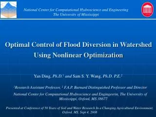
National Center for Computational Hydroscience and Engineering The University of Mississippi. Optimal Control of Flood Diversion in Watershed Using Nonlinear Optimization. Yan Ding, Ph.D. 1 and Sam S. Y. Wang, Ph.D. P.E. 2.

E N D
National Center for Computational Hydroscience and Engineering The University of Mississippi Optimal Control of Flood Diversion in Watershed Using Nonlinear Optimization Yan Ding, Ph.D.1and Sam S. Y. Wang, Ph.D. P.E.2 1Research Assistant Professor, 2 F.A.P. Barnard Distinguished Professor and Director National Center for Computational Hydroscience and Engingeerin, The University of Mississippi, Oxford, MS 38677 Presented at Conference of 50 Years of Soil and Water Research In a Changing Agricultural Environment, Oxford, MS, Sept 4, 2008
Outline • Introduction • Nonlinear Models for Forecasting Flood Events • Nonlinear Optimization Scheme for Finding the Optimal Flood Diversion Hydrograph to Mitigate Hazardous Storm Waters • Applications to a Variety of Flood Diversion Control Scenarios • Conclusions and Future Research Topics
An Example of Flood Diversion – The Bonnet Carre’ Spillway Flooded Street, Mississippi River Flood of 1927 The Bonnet Carré Spillway, the southern-most floodway in the Mississippi River and Tributaries system, has historically been the first floodway in the Lower Mississippi River Valley opened during floods. The USACE’s hydraulic engineers rely on discharge and gauge readings at Red River Landing, about 200 miles above New Orleans, to determine when to open the spillway. The discharge takes two days to reach the city from the landing. As flows increase, bays are opened at Bonnet Carré to divert them. The spillway (highlighted in green) stretches from the Mississippi River, at right, northward to Lake Ponchartrain, on the left of the photo.
Difficulties in Optimal Control of Open Channel Flow • Temporally/spatially non-uniform open channel flow Requires that a forecasting model can predict accurately complex water flows in space and time in single channel and channel network • Nonlinearity of flow control Nonlinear process control, Nonlinear optimization Difficulties to establish the relationship between control actions and responses of the hydrodynamic variables • Requirement of fast flow solver and optimization In case of fast propagation of flood wave, a very short time is available for predicting the flood flow at downstream. Due to the limited time for making decision of flood mitigation, it is crucial for decision makers to have a very efficient forecasting model and a control model.
Objectives • Theoretically, • Through adjoint sensitivity analysis, make nonlinear optimization capable of flow control in complex channel shape and channel network in watershed • Real-Time Nonlinear Adaptive Control Applicable to unsteady river flows • Establish a general numerical model for controlling hazardous floods so as to make it applicable to a variety of control scenarios • Flexible Control System; and a general tool for real-time flow control • For Engineering Applications, • Integrate the control model with the CCHE1D flow model, • Apply to practical problems
Integrated Watershed & Channel Network Modeling with CCHE1D Rainfall-Runoff Simulation Upland Soil Erosion (AGNPS or SWAT) Channel Network and Sub-basin Definition (TOPAZ) Digital Elevation Model (DEM) Channel Network Flow and Sediment Routing (CCHE1D) Dynamic Wave Model for Flood Wave Prediction where Q = discharge; Z=water stage; A=Cross-sectional Area; q=Lateral outflow; =correction factor; R=hydraulic radius n = Manning’s roughness A Typical Hydrograph by USGS • Boundary Conditions • Initial Conditions (Base Flows) • Internal Flow Conditions for Channel Network q(t)=?
Control Actions - Available Control Variables in Open Channel Flow • Control lateral flow at a certain location x0: Real-time flow diversion rate q(x0, t)at a spillway • Control lateral flow at the optimal location x: Real-time levee breaching rate q(x, t)at the optimal location • Control upstream discharge Q(0, t): real-time reservoir release • Control downstream stage Z(L, t): real-time gate operation • Control downstream discharge Q(L, t): real-time pump rate control • Control bed friction (roughness n):
An Objective Function for Flood Control Zobj To evaluate the discrepancy between predicted and maximum allowable stages, a weighted form is defined as where T=control duration; L = channel length; t=time; x=distance along channel; Z=predicted water stage; Zobj(x) =maximum allowable water stage in river bank (levee) (or objective water stage); x0= target location where the water stage is protective; = Dirac delta function
Mathematical Framework for Optimal Control • The optimazition is to find the control variable q satisfying a dynamic system such that where Q and Z are satisfied with the continuity equation and momentum equation, respectively (i.e., de Saint Venant Equations) • Local minimum theory : Necessary Condition: If n* is the true value, then J(n*)=0; Sufficient Condition: If the Hessian matrix 2J(n*) is positive definite, then n*is a strict local minimizer of f
Sensitivity Analysis- Establishing A Relationship between Control Actions and System Variables • Compute the gradient of objective function, q(X, q), i.e., sensitivity of control variable through 1. Influence Coefficient Method(Yeh, 1986): Parameter perturbation trial-and-error; lower accuracy 2. Sensitivity Equation Method (Ding, Jia, & Wang, 2004) Directly compute the sensitivity ∂X/∂q by solving the sensitivity equations Drawback: different control variables have different forms in the equations, no general measures for system perturbations; The number of sensitivity equations = the number of control variables. Merit: Forward computation, no worry about the storage of codes 3. Adjoint Sensitivity Method (Ding and Wang, 2003) Solve the governing equations and their associated adjoint equations sequentially. Merit: general measures for sensitivity, limited number of the adjoint equations (=number of the governing equations) regardless of the number of control variables. Drawback: Backward computation, has to save the time histories of physical variables before the computation of the adjoint equations.
Variational Analysis- To Obtain Adjoint Equations Extended Objective Function where A and Q are the Lagrangian multipliers Necessary Condition on the conditions that Fig. Solution domain
Variation of Extended Objective Function where Top width of channel
Variations of J with Respect to Control Variables – Formulations of Sensitivities Lateral Outflow Upstream Discharge Downstream Section Area or Stage Bed Friction Remarks: Control actions for open channel flows may rely on one control variable or a rational combination of these variables. Therefore, a variety of control scenarios principally can be integrated into a general control model of open channel flow.
General Formulations of Adjoint Equations for the Full Nonlinear Saint Venant Equations According to the extremum condition, all terms multiplied by A and Q can be set to zero, respectively, so as to obtain the equations of the two Lagrangian multipliers, i.e, adjoint equations (Ding & Wang 2003)
Transversality Conditions and Boundary Conditions Considering the contour integral in J*, This term I needs to be zero. Transversality (Final) Conditions Backward Computation Upstream B.C. Downstream B.C. Fig. Solution domain
Internal Boundary Conditions – for Channel Network I.B.C.s of Flow Model I.B.C.s of Adjoint Equations Fig. Confluence
Numerical Techniques 1-D Time-Space Discretization (Preissmann, 1961) where and are two weighting parameters in time and space, respectively; t=time increment; x=spatial length Solver of the resulting linear algebraic equations (Pentadiagonal Matrix) Double Sweep Algorithm based on the Gauss Elimination
Minimization Procedures for Nonlinear Optimization • CG Method (Fletcher-Reeves method) (Fletcher 1987) The convergence direction of minimization is considered as the gradient of objective function. • Trust Region Method (e.g Sakawa-Shindo method) considering the first order derivative of performance function only, stable in most of practical problems (Ding et al 2004) • Limited-Memory Quasi-Newton Method (LMQN) Newton-like method, applicable for large-scale computation, considering the second order derivative of objective function (the approximate Hessian matrix) (Ding & Wang 2005) • Others
Minimization Procedures • Limited-Memory Quasi-Newton Method (LMQN) Newton-like method, applicable for large-scale computation (with a large number of control parameters), considering the second order derivative of objective function (the approximate Hessian matrix) Algorithms: BFGS (named after its inventors, Broyden, Fletcher, Goldfarb, and Shanno) L-BFGS (unconstrained optimization) L-BFGS-B (bound constrained optimization)
Limited-Memory Quasi-Newton Method (LMQN) (Basic Concept 1) Given the iteration of a line search method for parameter q qk+1 = qk + kdk k = the step length of line search sufficient decrease and curvature conditions dk = the search direction (descent direction) Bk = nnsymmetric positive definite matrix For the Steepest Descent Method: Bk = I Newton’s Method: Bk= 2J(nk) Quasi-Newton Method: Bk= an approximation of the Hessian 2J(nk)
Flow chart of Finding optimal control variable by using LMQN procedure • Three Major Modules • Flow Solver • Sensitivity Solver • Minimization Process
L-BFGS-B • The purpose of the L-BFGS-B method is to minimize the objective function J(q) , i.e., min J(q), subject to the following simple bound constraint, qmin q qmax, where the vectors qmin and qmax mean lower and upper bounds on the control variables. • L-BFGS-B is an extension of the limited memory algorithm (L-BFGS) (Liu & Nocedal, 1989) for bound constrained optimization (Byrd et al, 1995).
Flooding and Flood Control Levee Failure, 1993 flood. Missouri. Flood Gate, West Atchafalaya Basin, Charenton Floodgate, Louisiana
Control of Flood Diversion in A Single Channel – A Simplified Problem xc q(xc,t) = ? Objective Function
Optimal Control of Flood Diversion Rate ( Case 1) - A Hypothetic Single Channel Lateral Outflow A Triangular Hydrograph Cross-section Z0=3.5m * This value is used for solving adjoint equations
Optimal Lateral Outflow and Objective Function (Case 1) Optimal Outflow q Objective function and Norm of gradient of the function Iterations of optimal lateral outflow
Comparison of Water Stages in Space and Time (Case 1) Allowable Stage Z0=3.5 No Control Optimal Control of Lateral Outflow
Comparison of Discharge in Time and Space (Case 1) No Control Optimal Control of Lateral Outflow
Sensitivity ∂J/∂q(x,t) Fast searching Sensitivity of q in time and space at the 1st iteration Iterative history of sensitivity at the control point
Optimal Control of Lateral Outflow (Case 2) –Under the limitation of the maximum lateral outflow rate Z0=-3.5m Lateral Outflow q≤q0 Application of the quasi-Newton method with bound constraints (L-BFGS-B) Bound Constraints: Suppose that the maximum lateral outflow rate is specified due to the limited capacity of flood gate or pump station, e.g. q 50.0 m3/s
Optimal Lateral Outflow with Constraint Comparison of optimal lateral outflow rates between Case 1 and Case 2 Iterations of optimal lateral outflow
Controlled Stage and Discharge in the Channel (Case 2) Allowable stage Z0=3.5m Stage in time and space Discharge in time and space
Optimal Control of Lateral Outflows – Multiple Lateral Outflows (Case 3) Z0=3.5m q1 q2 q3 Condition of control: Suppose that there are three flood gates (or spillways) in upstream, middle reach, and downstream.
Optimal Lateral Outflow Rates in Three Diversions (Case 3) Optimal lateral outflow rates of three floodgates (Case 4) Optimal lateral outflow of only one gate (=q1) (Case 1)
Controlled Stage and Discharge by Three Diversions (Case 3) Allowable stage Z0=3.5m Stage in time and space Discharge in time and space
Comparisons of Diversion Percentages and Objective Functions 3
Optimal Control of One Lateral Outflow in a Channel Network (Case 5) 1 3 m 0 0 0 , 4 = 1 L L = 3 1 3 , 0 0 0 m 2 . o N l e n n a h C m 0 0 5 , 4 = L 2 Z0=3.5m q(t)=? Compound Channel Section Confluence
Optimal Lateral Outflow and Objective Function (Case 5: Channel Network)
Comparisons of Stages (Case 5) 1 3 m 0 0 0 , 4 = 1 L L = 3 1 3 , 0 0 0 m 2 . o N l e n n a h C m 0 0 5 , 4 = L 2
Comparisons of Discharges (Case 5) 1 3 m 0 0 0 , 4 = 1 L L = 3 1 3 , 0 0 0 m 2 . o N l e n n a h C m 0 0 5 , 4 = L 2 Discharge increased !! Discharge increased !!
Optimal Control of Multiple Lateral Outflows in a Channel Network (Case 6) 1 3 q1(t)=? m 0 0 0 , 4 = 1 L q2(t)=? Z0=3.5m L = 3 1 3 , 0 0 0 m 2 . o N l e n n a h C q3(t)=? m 0 0 5 , 4 = L 2 Compound Channel Section
Optimal Lateral Outflow Rates and Objective Function (Case 6) One Diversion Three Diversions Optimal lateral outflow rates at three diversions Comparison of objective function
Comparisons of Stages (Case 6) 1 3 m 0 0 0 , 4 = 1 L L = 3 1 3 , 0 0 0 m 2 . o N l e n n a h C m 0 0 5 , 4 = L 2
Comparisons of Discharges (Case 6) 1 3 m 0 0 0 , 4 = 1 L L = 3 1 3 , 0 0 0 m 2 . o N l e n n a h C m 0 0 5 , 4 = L 2
Allowable Elevations along the River and Rating Curve at Outlet Zobj (x) Z-Q
Optimal Control of One Flood Gate in River Flow Comparison of Stages Optimal diversion hydrograph Storm Hydrograph