Optimal control
Optimal control. T. F. Edgar Spring 2012. Optimal Control. Static optimization (finite dimensions) Calculus of variations (infinite dimensions) Maximum principle ( Pontryagin ) / minimum principle Based on state space models Min S.t. is given General nonlinear control problem.

Optimal control
E N D
Presentation Transcript
Optimal control T. F. Edgar Spring 2012
Optimal Control • Static optimization (finite dimensions) • Calculus of variations (infinite dimensions) • Maximum principle (Pontryagin) / minimum principle Based on state space models Min S.t. is given General nonlinear control problem
Special Case of • Minimum fuel: • Minimum time: • Max range : • Quadratic loss: Analytical solution if state equation is linear, i.e.,
“Linear Quadratic” problem - LQP • Note is not solvable in a realistic sense ( is unbounded), thus need control weighting in • E.g., • is a tuning parameter (affects overshoot)
Ex. Maximize conversion in exit of tubular reactor : Concentration : Residence time parameter In other cases, when and are deviation variables, Objective function does not directly relate to profit (See T. F. Edgar paper in Comp. Chem. Eng., Vol 29, 41 (2004))
Initial conditions (a) , or Set point change, is the desired (b) , impulse disturbance, (c) , model includes disturbance term
Other considerations: “open loop” vs. “closed loop” • “open loop”: optimal control is an explicit function of time, depends on -- “programmed control” • “closed loop”: feedback control, depends on , but not on . e.g., Feedback control is advantageous in presence of noise, model errors. Optimal feedback control arises from a specific optimal control problems, the LQP.
Derivation of Minimum Principle , have continuous 1st partial w.r.t. Form Lagrangian Multipliers: adjoint variables, costates
Define (Hamiltonian) () • Since is Lagrangian, we treat as unconstrained problem with variables: , , • Use variations: , , (for => original constraint, the state equation.)
Since , are arbitrary (), then (n equations. “adjoint equation”) , “optimality equation” for weak minimum , (n boundary conditions) If is specified, then Two point boundary value problem (“TPBVP”)
Example: (1st order transfer function) LQP , (but don’t know yet)
Free canonical equations (eliminate ) (1) ( is known) (2) , Combine (1) and (2), for , initially correct to reduce
Another example: (double integrator)
Free canonical equations (,coupled) Char. Equation: (4 roots, apply boundary condition)
Can motivate feedback control via discrete time, one step ahead Set , ( fixed) Feedback control
Continuous Time LQP , , ()
Free canonical equations ( given) ( given) Let (Riccati transformation) , let (feedback control) Then we have ODE in (1) (2)
Substitute Eq. (1) into Eq. (2): (RiccatiODE) ( backward time integration) At steady state, for , solve steady state equation. is symmetric,
Example , , , Plug into Riccati Equation (Steady state) Feedback Matrix:
Generally 3 ways to solve steady state Riccati Equation: (1) integration of ode’s steady state; (2) Newton-Raphson (non linear equation solver); (3) transition matrix (analytical solution).
Transition matrix approach Reverse time integration (Boundary Condition: at ): Let When , Partition exponential
(1) (2) Combine (1) and (2), factor out Fix integration , is fixed Boundary condition: Backward time integration of , then forward time integration
Integral Action (eliminate offset) • Add terms or to objective function Example: Augment state equation (new state variable) (new control variable) Calculate feedback control Integrate:
Second method: ; Optimal control: With more state variables, PID controller