Optimal Control Theory
Optimal Control Theory. Prof .P.L.H .Vara Prasad. Dept of Instrument Technology Andhra university college of Engineering. Overview of Presentation. What is control system Darwin theory Open and closed loops Stages of Developments of control systems Mathematical modeling

Optimal Control Theory
E N D
Presentation Transcript
Optimal Control Theory Prof .P.L.H .Vara Prasad Dept of Instrument Technology Andhra university college of Engineering
Overview of Presentation What is control system Darwin theory Open and closed loops Stages of Developments of control systems Mathematical modeling Stability analysis Dept of Inst Technology Andhra university college of Engineering
What is a control system ? A control system is a device or set of devices to manage, command, direct or regulate the behavior of other devices or systems. Dept of Inst Technology Andhra university college of Engineering
Darwin (1805) Feedback over long time periods is responsible for the evolution of species. vito volterra - Balance between two populations of fish(1860-1940) Norbert wiener - positive and negative feed back in biology (1885-1964) Dept of Inst Technology Andhra university college of Engineering
Open loop & closed loop “… if every instrument could accomplish its own work, obeying or anticipating the will of others … if the shuttle weaved and the pick touched the lyre without a hand to guide them, chief workmen would not need servants, nor masters slaves.” Hall (1907) : Law of supply and demand must distrait fluctuations Any control system- Letting is to fluctuate and try to find the dynamics. Dept of Inst Technology Andhra university college of Engineering
Closed loop Due to feed back Complex More stable Effect of non-linearity can be minimized by selection of proper reference signal and feed back components Open loop Accuracy depends on calibration. Simple. Less stable. Presence of non-linearities cause malfunctions
Effects of feedback System dynamics normal improved Time constant 1/a 1/(a+k) Effect of disturbance Direct -1/g(s)h(s) reduced Gain is high low gain G/(1+GH) If GH= -1 , gain = infinity Selection of GH is more important in finding stable low Band width high band width
Stages of Developments of control systems Dept of Inst Technology Andhra university college of Engineering
optimization Maximize the profit or to minimize the cost dynamic programming . Non linear optimal control
Unit step response of a control system Dept of Inst Technology Andhra university college of Engineering
Steady state errors for various types of instruments Dept of Inst Technology Andhra university college of Engineering
For Higher order systems Rouths –Hurwitz stability criterion & its application Dept of Inst Technology Andhra university college of Engineering
Locus of the Roots of Characteristic Equation Dept of Inst Technology Andhra university college of Engineering
Root Contour Dept of Inst Technology Andhra university college of Engineering
Nyquist plots Third order system First order system Second order system
Limitations of Conventional Control Theory Applicable only to linear time invariant systems. Single input and single output systems Don’t apply to the design of optimal control systems Complex Frequency domain approach Trial error basis Not applicable to all types of in puts Don't include initial conditions
State Space Analysis of Control Systems Definitions of State Systems Representation of systems Eigen values of a Matrix Solutions of Time Invariant System State Transition Matrix
Definitions State – smallest set of variables that determines the behavior of system State variables – smallest set of variables that determine the state of the dynamic system State vector – N state variables forming the components of vector Sate space – N dimensional space whose axis are state variables
Solutions of Time Invariant System Solution of Vector Matrix Differential Equation X|= Ax (for Homogenous System) is given by X(t) = eAt X(0) (1) Ø(t) = eAt = L -1 [ (sI-A)-1 ] (2)
Solutions of Time Invariant System…(Cont’d) Solution of Vector Matrix Differential Equation X|= Ax+Bu (for Non- Homogenous System) is given by X(t) = eAt X(0) +∫t0 e ^{A(t - T)} * Bu(T) dT
Optimal Control Systems Criteria Selection of Performance Index Design for Optimal Control within constraints
Performance Indices Magnitudes of steady state errors Types of systems Dynamic error coefficients Error performance indexes
Optimization of Control System State Equation and Output Equation Control Vector Constraints of the Problem System Parameters Questions regarding the existence of Optimal control
Controllability A system is Controllable at time t(0) if it is possible by means of an unconstrained control vector to transfer the System from any initial state Xt(0) to any other state in a finite interval of time. Consider X| = Ax+Bu then system is completely state controllable if the rank of the Matrix [ B | AB | …….An-1B ] be n.
Observability A system is said to be observable at time t(0) if, with the system in state Xt(0) it is possible to determine the state from the observation of output over a finite interval of time. Consider X| = Ax+Bu, Y=Cox then system is completely state observable if rank of N * M matrix [C* | A*C* | …… (A*)n-1 C*] is of rank n .
Liapunov Stability Analysis Phase plane analysis and describing function methods – applicable for Non-linear systems Applicable to first and second order systems Liapunov Stability Analysis is suitable for Non-linear and|or Time varying State Equations
Stability in the Sense of Liapunov Stable Equilibrium state Asymptotically Stable Unstable state