OPTIMAL CONTROL SYSTEMS

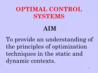
1. OPTIMAL CONTROL SYSTEMS AIM To provide an understanding of the principles of optimization techniques in the static and dynamic contexts.

2. LEARNING OBJECTIVES On completion of the module the student should be able to demonstrate:  - an understanding of the basic principles of optimization and the ability to apply them to linear and non-linear unconstrained and constrained static problems,  - an understanding of the fundamentals of optimal control.

3. LABORATORY WORK The module will be illustrated by laboratory exercises and demonstrations on the use of MATLAB and the associated Optimization and Control Tool Boxes for solving unconstrained and constrained static optimization problems and for solving linear quadratic regulator problems. ASSESSMENT  Via written examination.  MSc only - also laboratory session and report

4. PRINCIPLES OF OPTIMIZATION Typical engineering problem: You have a process that can be represented by a mathematical model. You also have a performance criterion such as minimum cost. The goal of optimization is to find the values of the variables in the process that yield the best value of the performance criterion.   Two ingredients of an optimization problem: (i) process or model (ii) performance criterion

5. Some typical performance criteria: ·maximum profit ·minimum cost ·minimum effort ·minimum error ·minimum waste ·maximum throughput ·best product quality  Note the need to express the performance criterion in mathematical form.

6. Static optimization: variables have numerical values, fixed with respect to time. Dynamic optimization: variables are functions of time.

7. Essential Features Every optimization problem contains three essential categories: 1.At least one objective function to be optimized 2.Equality constraints 3.Inequality constraints

8. x2 linear equality constraint nonlinear inequality constraints linear inequality constraint feasible region nonlinear inequality constraint x1 linear inequality constraint By a feasible solution we mean a set of variables which satisfy categories 2 and 3. The region of feasible solutions is called the feasible region.

9. An optimal solution is a set of values of the variables that are contained in the feasible region and also provide the best value of the objective function in category 1. For a meaningful optimization problem the model needs to be underdetermined.

10. Mathematical Description

11. Steps Used To Solve Optimization Problems • Analyse the process in order to make a list of all the variables. • Determine the optimization criterion and specify the objective function. • Develop the mathematical model of the process to define the equality and inequality constraints. Identify the independent and dependent variables to obtain the number of degrees of freedom. • If the problem formulation is too large or complex simplify it if possible. • Apply a suitable optimization technique. • Check the result and examine it’s sensitivity to changes in model parameters and assumptions.

12. Classification of optimization Problems Properties of f(x) ·single variable or multivariable ·linear or nonlinear ·sum of squares ·quadratic ·smooth or non-smooth ·sparsity

13. Properties of h(x) and g(x) ·simple bounds ·smooth or non-smooth ·sparsity ·linear or nonlinear ·no constraints

14. Properties of variables x • time variant or invariant • continuous or discrete • take only integer values • mixed

15. Obstacles and Difficulties • Objective function and/or the constraint functions may have finite discontinuities in the continuous parameter values. • Objective function and/or the constraint functions may be non-linear functions of the variables. • Objective function and/or the constraint functions may be defined in terms of complicated interactions of the variables. This may prevent calculation of unique values of the variables at the optimum.

16. Objective function and/or the constraint functions may exhibit nearly “flat” behaviour for some ranges of variables or exponential behaviour for other ranges. This causes the problem to be insensitive, or too sensitive. • The problem may exhibit many local optima whereas the global optimum is sought. A solution may be obtained that is less satisfactory than another solution elsewhere. • Absence of a feasible region. • Model-reality differences.

17. Typical Examples of Application static optimization • Plant design (sizing and layout). • Operation (best steady-state operating condition). • Parameter estimation (model fitting). • Allocation of resources. • Choice of controller parameters (e.g. gains, time constants) to minimise a given performance index (e.g. overshoot, settling time, integral of error squared).

18. dynamic optimization • Determination of a control signal u(t) to transfer a dynamic system from an initial state to a desired final state to satisfy a given performance index. • Optimal plant start-up and/or shut down. • Minimum time problems

19. BASIC PRINCIPLES OF STATIC optimization THEORY Continuity of Functions Functions containing discontinuities can cause difficulty in solving optimization problems. Definition: A function of a single variable x is continuous at a point xo if:

20. f(x) x f(x) is continuous, but f(x) is not. x If f(x) is continuous at every point in a region R, then f(x) is said to be continuous throughout R. f(x) is discontinuous.

21. at the extremum, the point is called a stationary point. Unimodal and Multimodal Functions A unimodal function f(x) (in the range specified for x) has a single extremum (minimum or maximum). A multimodal function f(x) has two or more extrema. There is a distinction between the global extremum(the biggest or smallest between a set of extrema) and local extrema(any extremum). Note: many numerical procedures terminate at a local extremum.

22. global max (not stationary) local max (stationary) stationary point (saddle point) local min (stationary) global min (stationary) f(x) x A multimodal function

23. For any multivariate function, the equation z = f(x) defines a surface in n+1 dimensional space . Multivariate Functions - Surface and Contour Plots We shall be concerned with basic properties of a scalar function f(x) of n variables (x1,...,xn). If n = 1, f(x) is a univariate function If n > 1, f(x) is a multivariate function.

24. In the case n = 2, the points z = f(x1,x2) represent a three dimensional surface. Let c be a particular value of f(x1,x2). Then f(x1,x2) = c defines a curve in x1 and x2 on the plane z = c. If we consider a selection of different values of c, we obtain a family of curves which provide a contour mapof the function z = f(x1,x2).

25. contour map of 4 5 3 6 z = 20 1.7 2 1.8 1.8 1.7 2 x2 1.0 saddle point 0.7 0.4 0.2 3 4 5 6 local minimum x1

28. Example: Surface and Contour Plots of “Peaks” Function

29. global max saddle local min x2 local max local max global min x1 multimodal!

31. The slope of f(x) at a point in the direction of the ith co-ordinate axis is Gradient Vector

32. The gradient vector at a point is normal to the the contour through that point in the direction of increasing f. increasing f At a stationary point: (a null vector)

33. Note: If is a constant vector, f(x) is then linear. e.g.

34. The function is strictly concaveif is replaced by >. A function is called convex (strictly convex) if is replaced by (<). Convex and Concave Functions A function is called concave over a given region R if:

35. f(x) x xa xb f(x) x xb xa concave function convex function

36. f(x) H(x) Hessian matrix For a multivariate function f(x) the conditions are:-

37. 1. all eigenvalues of H(x) are or 2. all principal determinants of H(x) are Tests for Convexity and Concavity H is +ve def (+ve semi def) iff H is -ve def (-ve semi def) iff Convenient tests: H(x) is strictly convex (+ve def) (convex) (+ve semi def)) if:

38. 1. all eigenvalues of H(x) are or 2. the principal determinants of H(x) are alternating in sign: H(x) is strictly concave (-ve def) (concave (- ve semi def)) if:

39. Example

40. xa xb convex region xa non convex region xb Convex Region A convex set of points exist if for any two points, xa and xb, in a region, all points: on the straight line joining xa and xb are in the set. If a region is completely bounded by concave functions then the functions form a convex region.

41. A condition N is necessary for a result R if R can be true only if N is true. A condition S is sufficient for a result R if R is true if S is true. A condition T is necessary and sufficient for a result R iff T is true. Necessary and Sufficient Conditions for an Extremum of an Unconstrained Function

42. There are two necessary and a single sufficient conditions to guarantee that x* is an extremum of a function f(x) at x = x*: 1. f(x) is twice continuously differentiable at x*. 2. , i.e. a stationary point exists at x*. 3. is +ve def for a minimum to exist at x*, or -ve def for a maximum to exist at x* 1 and 2 are necessary conditions; 3 is a sufficient condition. Note: an extremum may exist at x* even though it is not possible to demonstrate the fact using the three conditions.

43. Using (b) to eliminate x1 gives: (c) and substituting into (a) :- optimization with Equality Constraints Elimination of variables: example:

44. Then using (c): At a stationary point Hence, the stationary point (min) is: (1.071, 1.286)