Towards Strehl-Optimal Adaptive Optics Control
370 likes | 624 Vues
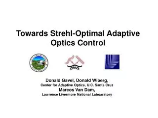
Towards Strehl-Optimal Adaptive Optics Control. Donald Gavel, Donald Wiberg, Center for Adaptive Optics, U.C. Santa Cruz Marcos Van Dam, Lawrence Livermore National Laboaratory. The goal of adaptive optics is to Maximize Strehl. Piston-removed atmospheric phase:. Phase correction by DM:.

Towards Strehl-Optimal Adaptive Optics Control
E N D
Presentation Transcript
Towards Strehl-Optimal Adaptive Optics Control Donald Gavel, Donald Wiberg, Center for Adaptive Optics, U.C. Santa Cruz Marcos Van Dam, Lawrence Livermore National Laboaratory
The goal of adaptive optics is to Maximize Strehl • Piston-removed atmospheric phase: • Phase correction by DM: vector of actuator commands vector of wavefront sensor readings actuator response functions • Max Strehl Þminimize residual wavefront variance (Marechal’saproximation) aperture averaged residual IPAM Workshop on Estimation and Control Problems in Adaptive Optics, Jan., 2004
Strehl-optimizing adaptive optics Define the cost function, J = mean square wavefront residual: Wavefront estimation and control problems are separable (proven on subsequent pages): where • JE is the estimation part: • JC is the control part: and is the conditional mean of the wavefront IPAM Workshop on Estimation and Control Problems in Adaptive Optics, Jan., 2004
The Conditional Mean The conditional probability distribution is defined via Bayes theorem: The conditional mean is the expected value over the conditional distribution: IPAM Workshop on Estimation and Control Problems in Adaptive Optics, Jan., 2004
Properties of the conditional mean 1. The conditional mean is unbiased: 2. The error in the conditional mean is uncorrelatedto the data it is conditioned on: 3. The error in the conditional mean is uncorrelated to the conditional mean: 4. The error in the conditional mean is uncorrelated to the actuator commands: IPAM Workshop on Estimation and Control Problems in Adaptive Optics, Jan., 2004
Proof that J = JE+JC (the estimation and control problems are separable) 0 0 IPAM Workshop on Estimation and Control Problems in Adaptive Optics, Jan., 2004
1) The conditional mean wavefront is the optimal estimate (minimizes JE) Proof: We show that any other wavefront estimate results in larger JE Let 0 for any Therefore, minimizes JE IPAM Workshop on Estimation and Control Problems in Adaptive Optics, Jan., 2004
Calculating the conditional mean wavefront given wavefront sensor measurements wavefront sensor operator: (average-gradient operator in the Hartmann slope sensor case) The measurement equation Measurement noise For Gaussian distributed f and n, it is straightforward to show (see next page) that the conditional mean of f must be a linear function of s: Cross-correlate both sides with s and solve for K (known as the “normal” equation) since so where IPAM Workshop on Estimation and Control Problems in Adaptive Optics, Jan., 2004
Aside: Proof that the conditional mean is a linear function of measurementsif the wavefront and measurement noise are Gaussian Measurement equation Measurement is a linear function of wavefront Bayesian conditional mean Gaussian distribution = maximum log-Likelihood of a-posteriori distribution = a linear (least squares) solution IPAM Workshop on Estimation and Control Problems in Adaptive Optics, Jan., 2004
2) The best-fit of the DM response functions to the conditional mean wavefront minimizes JC and where IPAM Workshop on Estimation and Control Problems in Adaptive Optics, Jan., 2004
Comparing to Wallner’s1 solution Combining the optimal estimator (1) and optimal controller (2) solutions gives Wallner’s “optimal correction” result: where • The two methods give the same result, a set of Strehl-optimizing actuator commands • The conditional mean approach separates the problem into two independent problems: • 1) statistically optimal estimation of the wavefront given noisy data • 2) deterministic optimal control of the wavefront to its optimal estimate given the deformable mirror’s actuator influence functions • We exploit the separation principle to derive a Strehl-optimizing closed-loop controller 1E. P. Wallner, Optimal wave-front correction using slope measurements, JOSA, 73, 1983. IPAM Workshop on Estimation and Control Problems in Adaptive Optics, Jan., 2004
The covariance statistics of f(x)(piston-removed phase over an aperture A) where IPAM Workshop on Estimation and Control Problems in Adaptive Optics, Jan., 2004
The g(x) function and a are “generic” under Kolmogorov statistics • Df(x) = 6.88(|x|/r0)5/3 • Circular aperture, diameter D • Factor out parameters 6.88(D/r0)5/3and integrals are computable numerically IPAM Workshop on Estimation and Control Problems in Adaptive Optics, Jan., 2004
Towards a Strehl-optimizing control law for adaptive optics Remember our goal is to maximize Strehl = minimize wavefront variance in an adaptive optics system • But adaptive optic systems measure and control the wavefront in closed loop at sample times that are short compared to the wavefront correlation time. • So the optimum controller uses the conditional mean, conditioned on alltheprevious data: IPAM Workshop on Estimation and Control Problems in Adaptive Optics, Jan., 2004
We need to progress the conditional mean through time (the Kalman filter2 concept) • Take a conditional mean at time t-1 and progress it forward to time t • Take data at time t • Instantaneously update the conditional mean, incorporating the new data • Progress forward to time step t+1 • etc. 2Kalman, R.E., A New Approach to Linear Filtering and Prediction Problems, J. Basic Eng.,Trans. ASME, 82,1, 1960. IPAM Workshop on Estimation and Control Problems in Adaptive Optics, Jan., 2004
Kalman filtering new data new data Update Update Time progress Time progress . . . . . . IPAM Workshop on Estimation and Control Problems in Adaptive Optics, Jan., 2004
Problems with calculating and progressing the conditional mean of an atmospheric wavefront through time • The wavefront is defined on a Hilbert Space (continuous domain) at an infinite number of points, xÎ A (A = the aperture). • The progression of wavefronts with time is not a well-defined process (Taylor’s frozen flow hypothesis, etc.) • In addition to the estimate, the estimate’s error covariance must be updated at each time step. In the Hilbert Space, these are covariance bi-functions: ct (x,x’)=<ft(x),ft(x’)>, x Î A, x’ Î A. IPAM Workshop on Estimation and Control Problems in Adaptive Optics, Jan., 2004
Justifying the extra effort of the optimal estimator/optimal controller • If is interesting to compare “best possible” solutions to what we are getting now, with “non-optimal” controllers • Determine if there is room for much improvement. • Gain insights into the sensitivity of optimal solutions to modeling assumptions (e.g. knowledge of the wind, Cn2 profile, etc.) • Preliminary analysis of tomographic (MCAO) reconstructors suggest that Weiner (statistically optimal) filtering may be necessary to keep the noise propagation manageable IPAM Workshop on Estimation and Control Problems in Adaptive Optics, Jan., 2004
Updating a conditional mean given new data Say we are given a conditional mean wavefront given previous wavefront measurements And a measurement at time t The residual is uncorrelated to previous measurements, Applying the normal equation on the two pieces of data etand st-1: 0 0 where Summarizing: IPAM Workshop on Estimation and Control Problems in Adaptive Optics, Jan., 2004
…written in Wallner’s notation • Estimate-update, given new data st: Hartmann sensor applied to the wavefront estimate Correlation of wavefront to measurement Correlation of measurement to itself • Covariance-update: where the estimate error is defined: IPAM Workshop on Estimation and Control Problems in Adaptive Optics, Jan., 2004
How it works in closed loop + Wavefront sensor Estimator - Best fit to DM + D Predictor IPAM Workshop on Estimation and Control Problems in Adaptive Optics, Jan., 2004
Closed-loop measurements need a correction term ^ …since what the wavefront sensor sees is not exactly the same as s - s, the wavefront measurement prediction error Measurement prediction error DM Fitting error Measurement prediction error = Hartmann sensor residual + DM Fitting error Þ (can be computed from the wavefront estimate and knowledge of the DM) (measured data) IPAM Workshop on Estimation and Control Problems in Adaptive Optics, Jan., 2004
Time-progressing the conditional mean ? how do we determine Given Example 1: On a finite aperture, the phase screen is unchanging and frozen in place Consequences: • Estimates corrections accrue (the integrator “has a pole at zero”) • If the noise covariance <vvT> is non-zero, then the updates cause the estimate error covariance to decrease monotonically with t. IPAM Workshop on Estimation and Control Problems in Adaptive Optics, Jan., 2004
Time-progressing the conditional mean Example 2: The aperture A is infinite, and the phase screen is frozen flow, with wind velocity w Consequence: • An infinite plane of phase estimates must be updated at each measurement IPAM Workshop on Estimation and Control Problems in Adaptive Optics, Jan., 2004
A A’ Time-progressing the conditional mean Example 3: The aperture A is finite, and the phase screen is frozen flow, with wind velocity w more on this approximation later as we might expect for x in the overlap region, AÙA’ The problem is to determine the progression operator, F(x,x’), for x in the newly blown in region, A- (A ÙA’ ) IPAM Workshop on Estimation and Control Problems in Adaptive Optics, Jan., 2004
“Near Markov” approximation The property where w is random noise uncorrelated to ft-1(x), is known as a Markov property. We see that if f obeyed a Markov property that is, the conditional mean on a finite sized aperture retains all of the relevant statistical information from the growing history of prior measurements. Phase f over the aperture however is not Markov, since some information in the “tail” portion, A’’ - (A’’ÙA’ ), which correlated to st-1, is dropped off and ignored. The fractal nature of Kolmogorov statistics does not allow us to write a Markov difference equation governing f on a finite aperture. We will nevertheless proceed assuming the Markov property since the effect of neglecting f in A’’ - (A’’ Ù A’ ) to estimates of f in A - (A ÙA’ ) is very small A A’’ A’ IPAM Workshop on Estimation and Control Problems in Adaptive Optics, Jan., 2004
Validity of approximating wind-blown Kolmogorov turbulence as near-Markov what is the effect of neglecting this point? using the estimate at this point To predict this point contribution of point in A’ contribution of neglected point in A’’ A A’ A’’ wind Information contained in points neglected by the near-Markov approximation is negligible IPAM Workshop on Estimation and Control Problems in Adaptive Optics, Jan., 2004
A A’ The progression operator from A’ to A We write the conditional mean of the wavefront in A, conditioned on knowing it in A’ G(x,x’’) solves (a normal equation) We can then say that Note: q(x) = 0 and G(x,x’) = d(x-x’-w) for x in the overlap AÙ A’ where q(x) is the error in the conditional mean f(x) - <f(x)|f(x’)>. q(x) is uncorrelated to the “data” (f(x’)) Also true in the overlap since q(x) = 0 there and, consequently since the measurement at t-1 depends only on f(x’) and random measurement noise. Then i.e. IPAM Workshop on Estimation and Control Problems in Adaptive Optics, Jan., 2004
A A’ In summary: The time-progression of the conditional mean is where F(x,x’) solves • If we assume the wavefront phase covariance function is constant or slowly varying with time, then the Green’s function F(x,x’) need only be computed infrequently (e.g. in slowly varying seeing conditions) • To solve this equation, we now need the cross-covariance statistics of the phase, piston-removed on two different apertures. IPAM Workshop on Estimation and Control Problems in Adaptive Optics, Jan., 2004
Cross-covariance of Kolmogorov phase, piston-removed on two different apertures A A’ Where c and c’ are the centers of the respective apertures, and as before also a “generic” function and IPAM Workshop on Estimation and Control Problems in Adaptive Optics, Jan., 2004
The error covariance must also progress, since it is used in the update formulas the error in the conditional mean is using and the error covariance is where Q is defined simply to preserve the Kolmogorov turbulence strength on the subsequent aperture IPAM Workshop on Estimation and Control Problems in Adaptive Optics, Jan., 2004
Simulations • Nominal parameters • D = 3m, d = 43cm (D/d = 7) • r0(l=0.5m)= 10cm ( r0(l=2m) @ d ) • w = 11m/s ´ 1 ms (w = D/300) • Noise = 0.1 arcsec rms • Simulations • Wallner’s equations strictly applied, even though the wind is blowing • Strehl-optimal controller • Optimal controller with update matrix, K, set at converged value (allows pre-computing error covariances) • Sensitivity to assumed r0 • Sensitivity to assumed wind speed • Sensitivity to assumed wind direction IPAM Workshop on Estimation and Control Problems in Adaptive Optics, Jan., 2004
Noise performance after convergence Single-step (Wallner) Strehl-optimal IPAM Workshop on Estimation and Control Problems in Adaptive Optics, Jan., 2004
Convergence time history K matrix fixed at converged value K matrix optimal at each time step IPAM Workshop on Estimation and Control Problems in Adaptive Optics, Jan., 2004
Sensitivity to r0 IPAM Workshop on Estimation and Control Problems in Adaptive Optics, Jan., 2004
Sensitivity to wind speed and direction IPAM Workshop on Estimation and Control Problems in Adaptive Optics, Jan., 2004
Conclusions • Kalman filtering techniques can be applied to better optimize the closed-loop Strehl of adaptive optics wavefront controllers • A-priori knowledge of r0 and wind velocity is required • Simulations show • Considerable improvement in performance over a single step optimized control law (Wallner) • Insensitivity to the exact knowledge of the seeing parameters over reasonably practical variations in these parameters IPAM Workshop on Estimation and Control Problems in Adaptive Optics, Jan., 2004