Understanding Price Changes and Their Effects on Consumption Patterns
Explore how price changes impact consumption of goods using budget lines, indifference curves, and demand curves in microeconomics. Learn how consumers adjust purchases at different price levels for goods X and Y.

Understanding Price Changes and Their Effects on Consumption Patterns
E N D
Presentation Transcript
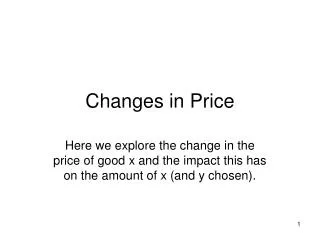
Changes in Price Here we explore the change in the price of good x and the impact this has on the amount of x (and y chosen).
Y Z C U3 B A U2 U1 X L M N
On slide 2 you see three budget lines and three indifference curves. The budget lines are different by the price of X. Say the consumer has $10 of income and the price of Y is $1. Then point Z would be the situation where the consumer buys only good y and the amount of y would be 10 units (the consumer shown won’t go to point Z, but at least it is possible.) Now if the price of x is $2 and the consumer spent all income on x then x would be 5. Let’s say this is the budget from Z to L. Then if the price of x is $1and the consumer spent all income on x then x would be 10. Let’s say this is the budget from Z to M. If the price of x is $0.50 (50 cent), and if all income is spent on x then x is 20. Let’s say this is the budget from Z to N. Conclusion about budget line when price of x changes: As price of x falls the budget line rotates counterclockwise around point Z, and as the price of x rises the budget line rotates clockwise around point Z.
Price consumption path In our graph on slide two let’s focus on a price of x decline. Initially the consumer can have utility U1 by maximizing utility at point A. Then when the price of x falls the consumer gets more utility at point B (utility U2) and we see in this example more x is taken because point B is to the right of point A and this means more x. If the price falls yet again the consumer moves to point C with more utility (U3) and even more x. I have drawn a line in the graph that connects all the consumer utility maximum points at each price of x, given income and the price of y. This line is called the price consumption path. The line is an indicator of where the consumer will go at various levels of the price of good x.
Demand curve we know and love Let’s review something. Budget ZL had the highest price of x in our story – let’s say the price is P1. Budget ZM had the 2nd highest price of x in our story – let’s say the price is P2. Budget ZN had the 3rd highest price of x in our story – let’s say the price is P3. When we take the price of x at each of these levels and keep track of the amount of x taken, we are getting the information we have always summarized in a graph of the demand curve. The demand curve is shown on the next slide. So, the demand curve for an individual is a result of the individuals search for maximum utility at each price of x given their taste and preference for x (and y) as shown by the indifference curves, given the price of y and given income.
Price of x P1 P2 P3 D x (quantity of x)