The Impact of Methane Clathrate Emissions on the Earth System

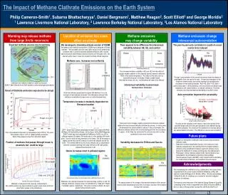
1. The Impact of Methane Clathrate Emissions on the Earth System Philip Cameron-Smith1, Subarna Bhattacharyya1, Daniel Bergmann1, Matthew Reagan2, Scott Elliott3 and George Moridis2 1 Lawrence Livermore National Laboratory, 2 Lawrence Berkeley National Laboratory, 3Los Alamos National Laboratory Warming may release methane from large Arctic reservoirs Location of emission has some effect on climate Methane emissions may change variability Methane emissions change interannual autocorrelation Expected methane sources due to warming We developed a chemistry-climate version of CESM There appears to be difference the interannual variability between AE, UE, and control The year-to-year auto correlation in southern ocean seems to be reduced We added a fast chemical mechanism to CESM that is designed to handle methane . We simulated over 600 years (after spinup) under present-day conditions with 1x and10x expected clathrate emissions (AE), and the same amount of extra emission spread uniformly over the globe (UE). We used an active ocean to see the coupled chemistry-climate response. PDF of annual temperatures Lag-1 autocorrelation coefficient 10x scenarios Global Arctic Methane conc. increases non-uniformly 10x scenarios Annual temperature (K) AE10x The increased methane variability in AE over UE (from the effect of synoptic weather patterns on the clathrate plumes) seems to affect the PDFs of the annual temperature. The effect on the Arctic isn’t as noticeable because it is already a highly variable region. Note that the mean, std. dev., and skewness all seem to be affected. 10x scenarios Lattitude Stolaroff, et al., 2012 The lag-1 autocorrelation of the annual time series shows the degree of predictability from one year to the next. It shows the importance of the long-term climate modes, and is also important for quantifying the uncertainty in time-series quantities. Red = AE, Blue = UE, black = control, black-dash = UE10x(fixedCH4), thin colored lines are Monte Carlo realizations with control statistics, to indicate confidence. The three methane runs show decreased predictability in southern ocean. UE10x(fixed) Clathrates are methane locked in a water ice structure. ESAS = East Siberian Arctic Shelf (methane under submerged permafrost) UE10x Interannual variability in zonal-mean temperature changes Onset of Clathrate emissions expected to be abrupt Ratio of standard deviations of zonal-mean surface temperatures to control Note that methane suppresses the specie that destroys it, so a 3x increase in total methane emissions (10x clathrates) produces 6-8x methane concentration increase over our control (present-day). Auto-correlation important for uncertainty Red Dots:Arctic Emission Black Dots: Control Uncertainty in surface temperature (K) Temperature increase is modestly dependent on Emission location 10x scenario Reagan, et al., 2011 Latitude Length of time-window (years) There seem to be changes roughly proportional to the level of global radiative forcing at several latitudes (indicated by arrows). In many cases the decreases are clearly related to sea-ice. In the zonal means, the difference between AE and UE is hard to distinguish from the uncertainty (1 sigma ~ 0.04). Note: the various 4xCO2 runs are very short, so their variability is much more uncertain. The dots are the variability in the means of each time window of the specified length within the 400 year simulations (with different starting years when possible). The circles are the standard error formula without any autocorrelation correction. The difference is due to auto-correlation. LEFT: Zonal mean surface temperature increase over control (AE=Red, UE=Blue, UE10x(fixedCH4)=Green, 2xCO2=Cyan, 4xCO2CMIP=Magenta). RIGHT: same data, but expressed as %difference for AE over UE for different regions (GL=globe, SP=south pole, LL=low latitudes, NP=north pole). The error bars are the uncertainty in the mean. The UE simulation is slightly warmer than the AE scenario for almost all latitudes except the Arctic. The modest difference in the Arctic seems to be a compensation between increased warming from extra methane in AE, with greater poleward heat transport in UE. This is the sediment response to a temperature ramp of 5K for 100 years. This emission rate is ~20% of global methane emissions. Most of the emission comes from 300-400m depth. Future plans • Couple our atmospheric methane model to ocean and permafrost methane codes. • Determine emission amplification factors, ie the amount of extra methane released due to the warming from the original methane emission (cross-amplification between reservoirs will also occur). • Assess the likelihood of runaway warming (aka, the clathrate gun). • Participate in future methane related model intercomparisons (we participated in the Atmospheric Chemistry-Climate Model Intercomparison Project (ACCMIP), which helped confirm and debug our model chemical behavior, and resulted in several papers). Fraction of methane that passes through ocean is uncertain, but could be large Variability decreases for El Nino and Sea-ice AE10x UE10x UE10x(fixedCH4) % methane released to atmosphere (no methanotrophs) Ozone increases most in polluted regions 10x scenario 50 m depth 150 m depth 10x scenarios Acknowledgements 2xCO2 4xCO2CMIP Sea-floor We acknowledge the contribution of our collaborators, who have primary responsibility for the ocean model (S.Elliott & M.Maltrud, LANL) and sediment model (M.Reagan & G. Moridis, LBNL). We also acknowledge J.Stolaroff (LLNL) for including us in a review for technical mitigation measures for methane. This research used resources of the National Energy Research Scientific Computing Center, which is supported by the Office of Science (BER) of the U.S. Dept. of Energy under Contract No. DE-AC02-05CH11231 Elliott, et al., 2010, 2011 Annual-mean surface ozone increase due to clathrate emission (vmr) Months since start of simulation Methane is an important precursor for chemical smog, and the 1x and 10x clathrate emissions increase ozone concentrations by ~5ppb and ~35ppb in polluted regions, respectively. The ozone increase is likely to be even greater during pollution events. The spatial pattern of the change in the standard deviation of the annual mean surface temperatures looks like it is mostly a function of the radiative forcing in the scenario. Methane is consumed in the ocean by methanotrophs. But, bubble plumes may inject methane to upper ocean levels which will allow faster release to the atmosphere. SPARC Meeting, Queenstown, 2014 This work is supported by the Earth System Modeling program of the Office of Science of the United States Department of Energy. This work was performed under the auspices of the U. S. Department of Energy by Lawrence Livermore National Laboratory under contract DE-AC52-07NA27344. LLNL-POST-648380