Object Recognition
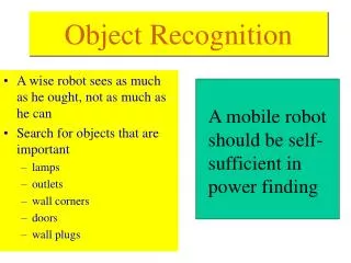
Object Recognition. A wise robot sees as much as he ought, not as much as he can Search for objects that are important lamps outlets wall corners doors wall plugs. A mobile robot should be self-sufficient in power finding. In any case, we need information reduction. Segmentation - Review.

Object Recognition
E N D
Presentation Transcript
Object Recognition • A wise robot sees as much as he ought, not as much as he can • Search for objects that are important • lamps • outlets • wall corners • doors • wall plugs A mobile robot should be self-sufficient in power finding
Segmentation - Review • Segmentation • Roughly speaking, segmentation is to partition the images into meaningful parts that are relatively homogenous in certain sense
Segmentation by Fitting a Model • One view of segmentation is to group pixels (tokens, etc.) belong together because they conform to some model • In many cases, explicit models are available, such as a line • Also in an image a line may consist of pixels that are not connectedor even close to each other
Why? • Image Processing • Canny Edge Detection • Hough Transforms • Monitor power level in robot’s batteries • When power goes low, interrupt actions • Search for the wall plug • Traverse over to it • Plug itself to it in.
How to design a n image processing system to solve this problem
Hough Transform Denoted by HT denoted by Standard HT, or SHT
Hough Transform • It locates straight lines • It locates straight line intervals • It locates circles • It locates algebraic curves • It locates arbitrary specific shapes in an image • But you pay progressively for complexity of shapes by time and memory usage
Hough Transform for circles * You need three parameters to describe a circle * * * * * * Vote space is three dimensional
Contours: Lines and Curves • Edge detectors find “edgels” (pixel level) • To perform imageanalysis : • edgels must be grouped into entities such as contours(higher level). • Canny does this to certain extent: the detector finds chains of edgels.
Hough Transform – cont. • Straight line case • Consider a single isolated edge point (xi, yi) • There are an infinite number of lines that could pass through the points • Each of these lines can be characterized by some particular equation
y x Line detection • Mathematical model of a line: Y = mx + n Y1=m x1+n Y2=m x2+n P(x1,y1) P(x2,y2) YN=m xN+n
slope Y = mx + n Y1=m x1+n m’ Y2=m x2+n y n n’ intercept m YN=m xN+n x Parameter Space Image and Parameter Spaces Y = m’x + n’ Image Space Line in Img. Space ~ Point in Param. Space
slope n y n = (-x) m + y intercept m P(x,y) Parameter Space x Hough Transform Technique • Given an edge point, there is an infinite number of lines passing through it (Vary m and n). • These lines can be represented as a line in parameter space.
Hough Transform Technique • Given a set of collinear edge points, each of them have associated a line in parameter space. • These lines intersect at the point (m,n) corresponding to the parameters of the line in the image space.
Hough Transform slope-intercept parametrization • An Edge Pixel in Real Space would vote into Hough Space all possible lines that contain that point y = kx + q • Continue to Add Votes for different Edge Pixels • Intersection gives Equation for line • Edge Detected Image (real space) • Hough Space
y = kx + q (x,y) - co-ordinates k - gradient q - y intercept Any straight line is characterized by k & q use : ‘slope-intercept’ or (k,q) space not (x,y) space (k,q) - parameter space (x,y) - image space can use (k,q) co-ordinates to represent a line HT - parametric representation
y x Looking at it backwards … Image space Y = mx + n Fix (m,n), Vary (x,y) - Line Y1=m x1+n Fix (x1,y1), Vary (m,n) – Lines thru a Point P(x1,y1)
m’ n n’ slope m intercept Looking at it backwards … Parameter space Y1=m x1+n Can be re-written as: n = -x1 m + Y1 Fix (-x1,y1), Vary (m,n) - Line n = -x1 m + Y1
Image Space Lines Points Collinear points Parameter Space Points Lines Intersecting lines Image Parameter Spaces
Hough Transform Philosophy • H.T. is a method for detecting straight lines, shapes and curves in images. • Main idea: • Map a difficult pattern problem into a simple peak detection problem
Hough Transform Technique • At each point of the (discrete) parameter space, count how many lines pass through it. • Use an array of counters • Can be thought as a “ parameter image” • The higher the count, the more edges are collinear in the image space. • Find a peak in the counter array • This is a “bright” point in the parameter image • It can be found by thresholding
Original HT designed to detect straight lines and curves Advantage - robustness of segmentation results segmentation not too sensitive to imperfect data or noise better than edge linking works through occlusion Any part of a straight line can be mapped into parameter space HT properties
Each edge pixel (x,y) votes in (k,q) space for each possible line through it i.e. all combinations of k & q This is called the accumulator If position (k,q) in accumulator has n votes n feature points lie on that line in image space Large n in parameter space, more probable that line exists in image space Therefore, find max n in accumulator to find lines Accumulators
Hough Transform • There are three problems in model fitting • Given the points that belong to a line, what is the line? • Which points belong to which line? • How many lines are there? • Hough transform is a technique for these problems • The basic idea is to record all the models on which each point lies and then look for models that get many votes
Hough Transform – cont. • Hough transform algorithm 1. Find all of the desired feature points in the image 2. For each feature point For each possibility i in the accumulator that passes through the feature point Increment that position in the accumulator 3. Find local maxima in the accumulator 4. If desired, map each maximum in the accumulator back to image space
Find all desired feature points in image space i.e. edge detect (low pass filter) Take each feature point increment appropriate values in parameter space i.e. all values of (k,q) for give (x,y) Find maxima in accumulator array Map parameter space back into image space to view results HT Algorithm
Practical Issues with This Hough Parameterization • The slope of the line is -<m< • The parameter space is INFINITE • The representation y = mx + n does not express lines of the form x = k
y P(x,y) y x x Solution: • Use the “Normal” equation of a line: Y = mx + n = x cos+y sin Is the line orientation Is the distance between the origin and the line
Consequence: • A Point in Image Space is now represented as a SINUSOID • = x cos+y sin
New Parameter Space for Hough based on trigonometric functions • Use the parameter space (, ) • The new space is FINITE • 0 < < D , where D is the image diagonal. • 0 < < • The new space can represent all lines • Y = k is represented with = k, =90 • X = k is represented with = k, =0
‘slope-intercept’ space has problem verticle lines k -> infinity q -> infinity Therefore, use (,) space = xcos + y sin = magnitude drop a perpendicular from origin to the line = angle perpendicular makes with x-axis Alternative line representation in (,) space
In (k,q) space point in image space == line in (k,q) space In (,) space point in image space == sinusoid in (,) space where sinusoids overlap, accumulator = max maxima still = lines in image space Practically, finding maxima in accumulator is non-trivial often smooth the accumulator for better results , space
Hough Transform Algorithm Input is an edge image (E(i,j)=1 for edgels) • Discretize and in increments of d and d. Let A(R,T) be an array of integer accumulators, initialized to 0. • For each pixel E(i,j)=1 and h=1,2,…T do • = i cos(h * d ) + j sin(h * d ) • Find closest integer k corresponding to r • Increment counter A(h,k) by one • Find local maxima in A(R,T)
Hough Transform Speed Up • If we know the orientation of the edge – usually available from the edge detection step • We fix theta in the parameter space and increment only one counter! • We can allow for orientation uncertainty by incrementing a few counters around the “nominal” counter.
Hough Transform – cont. • A better way of expressing lines for Hough transform