Efficient Self-Adjusting Tree Structures for Improved Searching Performance
Learn practical methods for optimizing data structures like trees and lists to enhance search speed. Discover self-adjusting and splay trees techniques for faster access and efficient search operations.

Efficient Self-Adjusting Tree Structures for Improved Searching Performance
E N D
Presentation Transcript
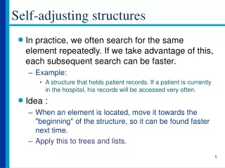
Self-adjusting structures • In practice, we often search for the same element repeatedly. If we take advantage of this, each subsequent search can be faster. • Example: • A structure that holds patient records. If a patient is currently in the hospital, his records will be accessed very often. • Idea : • When an element is located, move it towards the "beginning" of the structure, so it can be found faster next time. • Apply this to trees and lists.
Self-organizing lists • Move-to-front method • After the element is located, move it to the front of the list • Transpose method • After the element is located, swap it with its predecessor (unless it's already at the front). • Count method • Sort the list by the number of times each element has been accessed.
Self-adjusting trees • Main features: • Ignore balance requirement • When searching for an element, if it is found move it close to the root so that next time it will be found faster. • Time requirements: • Even though individual operations may take a lot of time, a sequence of operations overall behaves as if each operation was logarithmic. • In other words, inexpensive operations, such as searching for an element that happens to be very close to the root, cancel out expensive operations • Space requirements: • Better than balanced trees, since there is no need to store balance or height or color in the nodes.
Self-adjusting trees • Strategy #1 • If a node is accessed, move it towards the root by rotating once about its parent. • Strategy #2 (Splaying) • If a node is accessed, move it to the root through a sequence of rotations
Splay trees • Splay trees sacrifice balance in favor of taking advantage of the fact that in practice, only a small subset of the data items stored in the tree is responsible for a large percentage of the accesses. • Linear search time is now possible, but it does not happen very often because elements that are accessed frequently will soon be found very near or at the root of the tree. • When analyzing splay tree operations we perform amortized analysis. • In splay trees, it can be shown that a sequence of m operations takes at most O(mlgn) time, therefore the amortized cost of a single operation is O(lgn)
Splay trees: bottom-up splaying • Splaying = moving an item to the root via a sequence of rotations • In bottom-up splaying, we start at the node being accessed, and rotate from the bottom up along the access path until the node is at the root. • The nodes that are involved in the rotations are • the node being accessed (N) • its parent (P) • its grandparent (G)
Splay trees: bottom-up splaying • The rotation depends on the positions of the current node N, its parent P and its grandparent G • If N is the root, we are done • If P is the root, perform a single rotation P N N P • If P and N are both left or both right children, first rotate P • and then N as shown below N G P P P N G N G
Splay trees: bottom-up splaying • If P is a left child and N is a right child (or vice versa), first • rotate P and then N as shown below G G N P N P G N P
Splay trees: bottom-up splaying • Search • Once the node has been found, splay it • Insert • Insert the new node and immediately splay • Delete • Do a Search for the node to be deleted. It will end up at the root. Removing it will split the tree in two subtrees, the left (L) and the right (R) one • Find the maximum in L and splay it to the root of L. This root will have no right child • Make R a right child of L
8 8 6 9 7 7 6 9 3 8 6 6 9 3 7 1 4 7 9 3 3 1 4 1 4 1 4 Splay trees: bottom-up splaying • Example: delete 8
Splay trees: top-down splaying • In bottom-up splaying we traveled the tree down to locate the node to be splayed and then up to perform the splaying. • In top-down splaying • We travel the tree only once (down). • As we descend, we take the nodes that are found on the access path and move them out of the way while restructuring the “pieces” • In the end we put everything back together. • Time • The amortized time is the same (logarithmic) but in practice this method is faster.
Splay trees: top-down splaying • At any time during the splaying of a node x, we have three subtrees: • L = subtree containing nodes smaller than x, encountered on the access path towards x. • T = subtree containing x • Its root is always the current node on the search. • In the end, the root of T will be x. • R = subtree containing nodes larger than x, encountered on the access path towards x. • The tree is descended two levels at a time.
Splay trees: top-down splaying • In the figures that follow, the access path is indicated by a thicker line. • The tree is descended two levels at a time. We are interested in the current node, its child and its grandchild along the access path. • There are three cases: • zig • The target node is the child of the current node • zig-zig • The three nodes of interest form a straight line • zig-zag • The three nodes of interest form a zig-zag line
Splay trees: top-down splaying b a L R L A R a A B b B We are splaying node 'a'. Where should 'b' go? 'b' is greater than 'a', so it is attached to R Where in R should 'b' be attached? 'b' is smaller than every other node in R, so it should be placed in the lower left.
Splay trees: top-down splaying c a L R L A R b C a A B b c We are splaying node 'a'. Why did we rotate 'b' and 'c'? Even though we are not enforcing any balance restrictions, we still want to avoid a very imbalanced tree. The rotation helps in that (think of how R would look if we never rotated.) B C
Splay trees: top-down splaying c b L R L B R a C b A B a c A C We are splaying node 'b'. 'a' is smaller than 'b', and is placed in L 'c' is greater than 'b', and is placed in R