Download
1 / 20
200 likes | 216 Vues
Discover the complete nonlinear PBL solution for accurate surface pressure fields using scatterometer winds and modeling techniques in atmospheric science. Explore how to apply these solutions for improved weather and climate models.

E N D
Mike Freilich, Seawinds project scientist, was heard to say at my retirement party: Bob keeps us abreast of PBL applications, and what the ‘real’ PBL looks like, and its latest revelations. At times he gets impatient, as when he began one lecture with “Come on guys. Listen. Sometimes I feel like I’m casting pearls before swine.”
STOP Using the Ekman solution for Planetary Boundary Layer applications Using K-theory in modeling PBL fluxes
OK. • The nonlinear PBL solution requires a book (Brown, 1973) instead of a short paper (Ekman, 1905) • The nonlinear solution requires a quarter course instead of an hour lecture • The nonlinear solution requires a PBL measurement with at least an hour’s average or a 60-km flight path instead of a point measurement from a tower (point or short-time measurements often have significant errors)
But: • The nonlinear solution is complete (Foster, 1994, 2002). • The nonlinear solution has observational verification (SAR and scatterometer data, Brown 2005Comments on the synergism between the analytic PBL model and remote sensing data, Bound.-Layer Meteor., 116:187-199 ) • There is a version of the nonlinear solution ‘for dummies’ (Brown, 2005, 2002,Scaling Effects in Remote Sensing Applications and the Case of Organized Large Eddies, Canadian Jn. Remote Sensing, 28, 340-345, 2002,)
Hazards of taking measurements in the Rolls Station A Station B Hodograph from convergentzone of rolls Hodograph from center zone of rolls 1-km The OLE winds Station A 3 U 2 - 5 km 2 The Mean Wind Z/ 1 Station B V Mean Flow Hodograph RABrown 2004
Principle of The Red Queen • Named after the chess piece in Alice in Wonderland, - she moves faster & faster, in more complicated ways, yet Nothing Significant Changes. • Used in Evolution and Biology, mainly to describe the predator-prey relationship. • I’m mentioning this because I note that the principle seems to apply to modelling the turbulent PBL? (fantastically complicated turbulence models yet no better weather & climate models) {6-06: This left a wonderful hole for scatterometer winds to fill. Likewise for a lidar to fill some day.} R. A. Brown 2005 EMS (from EGU 2005), LIDAR 1/06
Surface Pressures from Space R. A. Brown 2005 AGU
The nonlinear solution applied to satellite surface winds yields accurate surface pressure fields. These data show: * Agreement between satellite and ECMWF pressure fields. This indicates that both the Scatterometer winds and the nonlinear PBL model (VG/U10) are accurate within 2 m/s. * A 3-month, zonally averaged offset angle <VG, U10> of 19° suggests the mean PBL state is near neutral (the angle predicted by the nonlinear PBL model). * Swath deviation angle observations can be used to infer thermal wind and stratification. * Higher winds are obtained from pressure gradients and used as surface truth (rather than from GCM or buoy winds). * VG (pressure gradients) rather than U10 could be used to initialize GCMs R. A. Brown 2006 AMS
NCEP real time forecasts use PBL model Even the best NCEP analysis, used as the first guess in the real time forecasts, is improved with the QuikScat surface pressure analyses.
This is the actual slp output from the uwpbl model using the 0543 UTC QuikSCAT pass
This is the actual output of the uwpbl model slp using the 0648 UTC QuikSCAT pass
This is a composite of two runs of the model using the 0549 QuikSCAT pass and the 0648 QuikSCAT pass.
This is the 0600 UTC Ocean Prediction Center hand drawn surface analysis superimposed over the GOES12 0615UTC Image.
This is the composite of three consecutive runs of the uwpbl model using the 0543, 0648 and 0834 QuikSCAT passes superimposed on the GOES 12 image from 0645 UTC
This is the Ocean Prediction Center hand drawn surface analysis 0526 0600 UTC with the surface vorticity field from the uwpbl model overlaid. The vorticity field is a composite of three passes (0543, 0648 and 0834 UTC); it shows the locations of the frontal zones well.
Improved 6/06 a 991 b 999 QuikSCAT 10 Jan 2005 0709 UTC GFS Sfc Analysis 10 Jan 2005 0600 UTC c d 984 996 982 996 OPC Sfc Analysis and IR Satellite Image 10 Jan 2005 0600 UTC UWPBL 10 Jan 2005 0600 UTC This example is from 10 January 2005 0600UTC. Numerical guidance from the 0600UTC GFS model run (a) indicated a 999 hPa low at 43N, 162E. QuikScat winds (b) suggested strong lows --- OPC analysis uses 996. UW-PBL analysis indicates 982.
Programs and Fields available onhttp://pbl.atmos.washington.eduQuestionsto rabrown, Ralph orjerome @atmos.washington.edu • Direct PBL model: PBL_LIB. (’75 -’05) An analytic solution for the PBL flow with rolls, U(z) = f( P, To , Ta , ) • The Inverse PBL model: Takes U10 field and calculates surface pressure field P (U10 , To , Ta , ) (1986 - 2005) • Pressure fields directly from the PMF: P (o) along all swaths (exclude 0 - 5° lat.?) (2001) (dropped in favor of I-PBL) • Global swath pressure fields for QuikScat swaths (with global I-PBL model) (2005) • Surface stress fields from PBL_LIB corrected for stratification effects along all swaths (2006) R. A. Brown 2006
1980 – 2005: Using surface wind as a lower boundary condition on a PBL model, considerable information about the atmosphere and the PBL has been inferred. • The symbiotic relation between surface backscatter data and the PBL model has been beneficial to both. • The PBL model has established superior ‘surface truth’ winds (or pressures) for the satellite model functions. • Satellite data have proven that the nonlinear PBL solution with OLE is observed most of the time. R. A. Brown 2006 AMS