Biostat 200 Lecture 8
600 likes | 766 Vues
Biostat 200 Lecture 8. Where are we. Types of variables Descriptive statistics and graphs Probability Confidence intervals for means and proportions Hypothesis testing for means and medians and proportions (alone or grouped by a categorical variable)

Biostat 200 Lecture 8
E N D
Presentation Transcript
Where are we • Types of variables • Descriptive statistics and graphs • Probability • Confidence intervals for means and proportions • Hypothesis testing for means and medians and proportions (alone or grouped by a categorical variable) • Today: Testing for categorical variables grouped by another categorical variable • Lectures 9+10: Correlations and linear regression • Lecture 11: Logistic regression
Assumptions of hypothesis tests • For t-test and ANOVA, the underlying distribution of the random variable being measured (X) should be approximately normal • In reality the t-test is rather robust, so with large enough sample size and without very large outliers, it is ok to use the t-test • For the ANOVA, the variance of the subgroups should be approximately equal • For the Wilcoxon Rank Sum Test and the Kruskal-Wallis Test the underlying distributions must have the same basic shape
Categorical outcomes • With the exception of the proportion test, all the previous tests were for comparing numerical outcomes and categorical predictors • E.g., CD4 count by alcohol consumption • Hours of sleep by sex • We often have dichotomous outcomes and predictors • E.g. Had at least one cold in the prior month by sex
We can make tables of the number of observations falling into each category • These are called contingency tables • E.g. At least one cold by sex . tab coldany sex | Biological sex at | birth coldany | Male Female | Total -----------+----------------------+---------- No | 140 175 | 315 Yes | 74 116 | 190 -----------+----------------------+---------- Total | 214 291 | 505
Contingency tables • Often summaries of counts of disease versus no disease and exposed versus not exposed • Frequently 2x2 but can generalize to n x k • n rows, k columns • Note that Stata sorts on the numeric value, so for 0-1 variables the disease state will be the 2nd row
Contingency tables • Contingency tables are usually summaries of data that originally looked like this.
. list coldany sex in 1/20 +------------------+ | coldany sex | |------------------| 1. | Yes Female | 2. | No Male | 3. | No Female | 4. | No Female | 5. | No Female | |------------------| 6. | No Female | 7. | Yes Male | 8. | No Male | 9. | Yes Male | 10. | No Male | |------------------| 11. | Yes Male | 12. | Yes Male | 13. | No Male | 14. | No Female | 15. | Yes Male | |------------------| 16. | Yes Male | 17. | Yes Female | 18. | Yes Male | 19. | Yes Female | 20. | Yes Male | +------------------+ . list coldany sex in 1/20, nolabel +---------------+ | coldany sex | |---------------| 1. | 1 1 | 2. | 0 0 | 3. | 0 1 | 4. | 0 1 | 5. | 0 1 | |---------------| 6. | 0 1 | 7. | 1 0 | 8. | 0 0 | 9. | 1 0 | 10. | 0 0 | |---------------| 11. | 1 0 | 12. | 1 0 | 13. | 0 0 | 14. | 0 1 | 15. | 1 0 | |---------------| 16. | 1 0 | 17. | 1 1 | 18. | 1 0 | 19. | 1 1 | 20. | 1 0 | +---------------+
We want to know whether the incidence of colds varies by gender. • We could test the null hypothesis that the cumulative incidence of ≥1 cold in males equals that of females. The cumulative incidence is a proportion. H0: pmales= pfemales HA: pmales≠ pfemales • This is the test of proportions from Lecture 6
The Proportion test . prtest coldany, by(sex) Two-sample test of proportion Male: Number of obs = 214 Female: Number of obs = 291 ------------------------------------------------------------------------------ Variable | Mean Std. Err. z P>|z| [95% Conf. Interval] -------------+---------------------------------------------------------------- Male | .3457944 .0325132 .2820698 .409519 Female | .3986254 .0287018 .342371 .4548798 -------------+---------------------------------------------------------------- diff | -.052831 .0433693 -.1378333 .0321712 | under Ho: .0436248 -1.21 0.226 ------------------------------------------------------------------------------ diff = prop(Male) - prop(Female) z = -1.2110 Ho: diff = 0 Ha: diff < 0 Ha: diff != 0 Ha: diff > 0 Pr(Z < z) = 0.1129 Pr(|Z| < |z|) = 0.2259 Pr(Z > z) = 0.8871
There are other methods to do this (chi-square test) • Why? • These methods are more general – can be used when you have more than 2 levels in either variable • We will start with the 2x2 example however
Overall, the cumulative incidence of least one cold in the prior month is 190/505=.3762 This is the marginal probability of having a cold • There were 214 males and 291 females • Under the null hypothesis, the expected cumulative incidence in each group is the overall cumulative incidence • So the expected number of colds: Males 214*.3762=80.5 Females: 291*.3762=109.5
We can also calculate the expected number with no colds under the null hypothesis of no difference • Males: 214*(1-.3762) = 133.5 • Females: 291*(1-.3862) = 181.5 • We can make a table of the expected counts EXPECTED COUNTS UNDER THE NULL HYPOTHESIS | sex coldany | Male Female | Total -----------+----------------------+---------- No | 133.5 181.5 | 315 Yes | 80.5 109.5 | 190 -----------+----------------------+---------- Total | 214 291 | 505 Observed data . tab coldany sex | Biological sex at | birth coldany | Male Female | Total -----------+----------------------+---------- No | 140 175 | 315 Yes | 74 116 | 190 -----------+----------------------+---------- Total | 214 291 | 505
The Chi-square test compares the observed frequency (O) in each cell with the expected frequency (E) under the null hypothesis of no difference • The differences O-E are squared, divided by E, and added up over all the cells • The sum of this is the test statistic and follows a chi-square distribution
Chi-square test of independence • The chi-square test statistic (for the test of independence in contingency tables) for a 2x2 table (dichotomous outcome, dichotomous exposure) • i is the index for the cells in the table – there are 4 cells • This test statistic is compared to the chi-square distribution with 1 degree of freedom
Chi-square test of independence • The chi-square test statistic for the test of independence in an nxk contingency table is • This test statistic is compared to the chi-square distribution • The degrees of freedom for the this test are (n-1)*(k-1), so for a 2x2 there is 1 degree of freedom • n=the number of rows; k=the number of columns in the nxk table • The chi-square distribution with 1 degree of freedom is actually the square of a standard normal distribution • Expected cell sizes should all be >1 and fewer than 20% should be <5 • The Chi-square test is for two sided hypotheses
Chi-square distribution Mean = degrees of freedom Variance = 2*degrees of freedom
Chi-square test of independence • For the example, the chi-square statistic for our 2x2 is (140-133.5)2 /133.5 + (175-181.5)2 /181.5 + (74-80.5)2 /80.5 + (116-109.5)2 /109.5 . di (140-133.5)^2 /133.5 + (175-181.5)^2 /181.5 + (74-80.5)^2 /80.5 + (116-109.5)^2 /109.5 1.4599512 • There is 1 degree of freedom • Probability of observing a chi-square value of 1.45 with 1 degree of freedom . di chi2tail(1,1.45995) .22693808 Fail to reject the null hypothesis of independence
tab coldany sex, chi | Biological sex at | birth coldany | Male Female | Total -----------+----------------------+---------- 0 | 140 175 | 315 1 | 74 116 | 190 -----------+----------------------+---------- Total | 214 291 | 505 Pearson chi2(1) = 1.4666 Pr = 0.226 p-value Test statistic (df)
If you want to see the row or column percentages, use row or col options . . tab coldany sex, row col chi expected +--------------------+ | Key | |--------------------| | frequency | | expected frequency | | row percentage | | column percentage | +--------------------+ | Biological sex at | birth coldany | Male Female | Total -----------+----------------------+---------- 0 | 140 175 | 315 | 133.5 181.5 | 315.0 | 44.44 55.56 | 100.00 | 65.42 60.14 | 62.38 -----------+----------------------+---------- 1 | 74 116 | 190 | 80.5 109.5 | 190.0 | 38.95 61.05 | 100.00 | 34.58 39.86 | 37.62 -----------+----------------------+---------- Total | 214 291 | 505 | 214.0 291.0 | 505.0 | 42.38 57.62 | 100.00 | 100.00 100.00 | 100.00 Pearson chi2(1) = 1.4666 Pr = 0.226
Because we using discrete cell counts to approximate a chi-squared distribution, for 2x2 tables some use the Yatescorrection • Not computed in Stata
Lexicon • When we talk about the chi-square test, we are saying it is a test of independence of two variables, usually exposure and disease. • We also say we are testing the “association” between the two variables. • If the test is statistically significant (p<0.05 if =0.05), we often say that the two variables are “not independent” or they are “associated”.
Test of independence • For small cell sizes in 2x2 tables, use the Fisher exact test • It is based on a discrete distribution called the hypergeometric distribution • For 2x2 tables, you can choose a one-sided or two-sided test . tab coldany sex, chi exact | Biological sex at | birth coldany | Male Female | Total -----------+----------------------+---------- 0 | 140 175 | 315 1 | 74 116 | 190 -----------+----------------------+---------- Total | 214 291 | 505 Pearson chi2(1) = 1.4666 Pr = 0.226 Fisher's exact = 0.229 1-sided Fisher's exact = 0.132
Comparison to test of two proportions . prtest coldany, by(sex) Two-sample test of proportion Male: Number of obs = 214 Female: Number of obs = 291 ------------------------------------------------------------------------------ Variable | Mean Std. Err. z P>|z| [95% Conf. Interval] -------------+---------------------------------------------------------------- Male | .3457944 .0325132 .2820698 .409519 Female | .3986254 .0287018 .342371 .4548798 -------------+---------------------------------------------------------------- diff | -.052831 .0433693 -.1378333 .0321712 | under Ho: .0436248 -1.21 0.226 ------------------------------------------------------------------------------ diff = prop(Male) - prop(Female) z = -1.2110 Ho: diff = 0 Ha: diff < 0 Ha: diff != 0 Ha: diff > 0 Pr(Z < z) = 0.1129 Pr(|Z| < |z|) = 0.2259 Pr(Z > z) = 0.8871 --- For 2x2 tables the chi-square statistic is equal to the z statistic squared . di 1.2110^2 1.466521
Chi-square test of independence • The chi-square test can be used for more than 2 levels of exposure (with a dichotomous outcome) • The null hypothesis is p1 = p2 = ... = pk • The alternative hypothesis is that not all the proportions are the same • Note that, like ANOVA, a statistically significant result does not tell you which level differed from the others • Also when you have more than 2 groups, all tests are 2-sided • The degrees of freedom for the test are k-1
Chi-square test of independence tab coldany race4, col chi exact +-------------------+ | Key | |-------------------| | frequency | | column percentage | +-------------------+ Enumerating sample-space combinations: stage 4: enumerations = 1 stage 3: enumerations = 13 stage 2: enumerations = 120 stage 1: enumerations = 0 | race4 coldany | White, Ca Asian/PI Black, Af Other | Total -----------+--------------------------------------------+---------- 0 | 191 52 31 40 | 314 | 63.67 55.91 58.49 68.97 | 62.30 -----------+--------------------------------------------+---------- 1 | 109 41 22 18 | 190 | 36.33 44.09 41.51 31.03 | 37.70 -----------+--------------------------------------------+---------- Total | 300 93 53 58 | 504 | 100.00 100.00 100.00 100.00 | 100.00 Pearson chi2(3) = 3.2780 Pr = 0.351 Fisher's exact = 0.353
Another way to state the null hypothesis for the chi-square test: • Factor A is not associated with Factor B • The alternative is • Factor A is associated with Factor B • For more than 2 levels of the outcome variable this would make the most sense • The degrees of freedom are (r-1)*(c-1) (r=rows, c=columns)
Note that this is a 3x4 table, so the chi-square test has 2x3=6 degrees of freedom . . . . tab cold3 race4, col chi exact +-------------------+ | Key | |-------------------| | frequency | | column percentage | +-------------------+ RECODE of | race4 cold | White, Ca Asian/PI Black, Af Other | Total -----------+--------------------------------------------+---------- None | 191 52 31 40 | 314 | 63.67 55.91 58.49 68.97 | 62.30 -----------+--------------------------------------------+---------- One | 91 30 14 17 | 152 | 30.33 32.26 26.42 29.31 | 30.16 -----------+--------------------------------------------+---------- 2 or more | 18 11 8 1 | 38 | 6.00 11.83 15.09 1.72 | 7.54 -----------+--------------------------------------------+---------- Total | 300 93 53 58 | 504 | 100.00 100.00 100.00 100.00 | 100.00 Pearson chi2(6) = 11.4600 Pr = 0.075 Fisher's exact = 0.081
Paired dichotomous data • Matched pairs • Matched case-control study • Before and after data • You cannot just put each individual into an exposure and disease box, because then you would lose the benefits of pairing (and the observations would not be independent!) • Instead you have a table that tabulates each of the 4 possible states for each pair
Paired dichotomous data • For a 1:1 matched case/control study, in all pairs, 1 has the disease (case) and 1 does not (control). The table then counts the number of pairs in which • 1. Both were exposed • 2. Neither were exposed • 3. The case was exposed, the control was not • 4. The case was not exposed, the control was exposed
Case-control studyHIV positives on ART in Uganda • The study question was: Is alcohol consumption associated with treatment failure? • The null hypothesis is that alcohol consumption is not associated with treatment failure • Cases: • HIV viral load after 6 months of ART >400 cells/mm3 • Controls: • HIV viral load <400 • Matched on sex, duration on treatment, and treatment regimen class
. tab lastalc_case lastalc_control lastalc_ca | lastalc_control se | No Yes | Total -----------+----------------------+---------- No | 11 3 | 14 Yes | 9 4 | 13 -----------+----------------------+---------- Total | 20 7 | 27 . list id lastalc_case lastalc_control +-------------------------------+ | id lastal~e lastal~l | |-------------------------------| 1. | MBO1007 1 0 | 2. | MBO1009 1 1 | 3. | MBO1012 0 0 | 4. | MBO1019 1 0 | 5. | MBO1020 0 0 | |-------------------------------| 6. | MBO1021 0 1 | 7. | MBO1022 1 1 | 8. | MBO1028 1 0 | 9. | MBO1030 0 0 | 10. | MBO1035 0 0 | |-------------------------------| 11. | MBO1039 1 1 | 12. | MBO1043 0 1 | 13. | MBO1044 1 0 | 14. | MBO1046 1 0 | 15. | MBO1047 1 0 | |-------------------------------| 16. | MBO1048 0 0 | 17. | MBO1049 0 0 | 18. | MBO1055 0 0 | 19. | MBO1056 1 0 | 20. | MBO1057 0 0 | |-------------------------------| 21. | MBO1058 1 0 | 22. | MBO1060 0 0 | 23. | MBO1061 1 1 | 24. | MBO1062 0 0 | 25. | MBO1027 1 0 | |-------------------------------| 26. | MBO1036 0 1 | 27. | MBO1032 0 0 | +-------------------------------+ Data are in “treatment outcomes case control.dta”
The test statistic is • r and s are the number of discordant pairs • Concordant pairs provide no information • Under the null hypothesis, r and s would be equal • This statistic has an approximate chi-square distribution with 1 degree of freedom • The test is called McNemar’s test • The -1 is a continuity correction, not all versions of the test use this, some use .5
r=9, s=3 • Test statistic = (9-3-1)^2/12 = 2.083 . di chi2tail(1,2.083) .14894719 • Test statistic = (6)^2/12 = 3 (Not using the continuity correction) di chi2tail(1,3) .08326452
In Stata, use mcc for Matched Case Control mcc case_exposed control_exposed . . mcc lastalc_case lastalc_control | Controls | Cases | Exposed Unexposed | Total -----------------+------------------------+------------ Exposed | 4 9 | 13 Unexposed | 3 11 | 14 -----------------+------------------------+------------ Total | 7 20 | 27 McNemar's chi2(1) = 3.00 Prob > chi2 = 0.0833 Exact McNemar significance probability = 0.1460 Proportion with factor Cases .4814815 Controls .2592593 [95% Conf. Interval] --------- -------------------- difference .2222222 -.0518969 .4963413 ratio 1.857143 .9114712 3.78397 rel. diff. .3 .0159742 .5840258 odds ratio 3 .7486845 17.228 (exact)
Use mcci if you only have the table, not the raw data mcci #both_exposed #case_exposed_only #control_exposed_only #neither_exposed . mcci 4 9 3 11 | Controls | Cases | Exposed Unexposed | Total -----------------+------------------------+------------ Exposed | 4 9 | 13 Unexposed | 3 11 | 14 -----------------+------------------------+------------ Total | 7 20 | 27 McNemar's chi2(1) = 3.00 Prob > chi2 = 0.0833 Exact McNemar significance probability = 0.1460 Proportion with factor Cases .4814815 Controls .2592593 [95% Conf. Interval] --------- -------------------- difference .2222222 -.0518969 .4963413 ratio 1.857143 .9114712 3.78397 rel. diff. .3 .0159742 .5840258 odds ratio 3 .7486845 17.228 (exact)
Note that the McNemar test is only for MATCHED case/control data • It is quite possible to collect unmatched case control data. Then you analyze using the chi-square methods presented earlier.
Paired dichotomous data • For before and after data, the pairs are the individual participant, and the four outcomes might be: 1. “Yes” before + “Yes” after (no change) 2. “No” before + “No” after (no change) 3. “Yes” before + “No” after 4. “No” before + “Yes” after • E.g. Reporting alcohol consumption before and after being consented to a study in which blood and urine will be tested for an alcohol biomarker
Self-reported alcohol consumption in UgandaMcNemar’s test for paired data • Null hypothesis: The groups change their self-reported alcohol consumption equally • use auditc_2studies.dta", clear • recode auditc_s1 (0 = 0 "None") (1/7 = 1 "Any"), gen(alc3mos_s1) • recode auditc_s2 (0 = 0 "None") (1/7 = 1 "Any"), gen(alc3mos_s2) . tab alc3mos_s1 alc3mos_s2 RECODE of | auditc_s1 | (auditc | from | closest | prev uarto | RECODE of auditc_s2 on/b4 | (AUDIT-C scores) tmtout) | None Any | Total -----------+----------------------+---------- None | 17 7 | 24 Any | 0 4 | 4 -----------+----------------------+---------- Total | 17 11 | 28
Matched case-control study command . . mcc alc3mos_s1 alc3mos_s2 | Controls | Cases | Exposed Unexposed | Total -----------------+------------------------+------------ Exposed | 4 0 | 4 Unexposed | 7 17 | 24 -----------------+------------------------+------------ Total | 11 17 | 28 McNemar's chi2(1) = 7.00 Prob > chi2 = 0.0082 Exact McNemar significance probability = 0.0156 Proportion with factor Cases .1428571 Controls .3928571 [95% Conf. Interval] --------- -------------------- difference -.25 -.4461015 -.0538985 ratio .3636364 .1664008 .7946562 rel. diff. -.4117647 -.7741991 -.0493304 odds ratio 0 0 .693814 (exact)
Comparison of disease frequencies across groups • The chi-square test and McNemar’s test are tests of independence • They do not give us an estimate of how much the two groups differ, i.e. how much the disease outcome varies by the exposure variable • We use odds ratios (OR) and relative risks (RR) as measures of ratios of disease outcome (given exposure or lack of exposure) • The odds ratio and the relative risk are just two examples of “measures of association”
Comparison of disease frequencies – relative risk • Risk ratio (or relative risk or relative rate) = P (disease | exposed) / P(disease | unexposed) = Re / Ru= a/(a+c) / b/(b+d)
Comparison of disease frequencies – relative risk • Note that you cannot calculate this entity when you have chosen your sample based on disease status • I.e. Case-control study – you have fixed a prior the probability of disease! Relative risk is a NO GO! • You can calculate it but it won’t have any meaning…
Odds • If an event occurs with probability p, the odds of the event are p/(1-p) to 1 • If an event has probability .5, the odds are 1:1 • Conversely, if the odds of an event are a:b, the probability of a occurring is a/(a+b) • The odds of horse A winning over horse B winning are 2:1 the probability of horse A winning is .667.
Odds ratio • Odds of disease among the exposed persons = P(disease | exposed) / (1-P(disease | exposed)) = [ a / (a + c) ] / [ c / (a + c) ] = a/c • Odds of disease among the unexposed persons = P(disease | unexposed) / (1-P(disease | unexposed)) = [ b / (b + d) ] / [ d / (b + d) ] = b/d • Odds ratio = a/c / b/d = ad/bc
Odds ratio note • Note that the odds ratio is also equal to [ P(exposed | disease)/(1-P(exposed |disease) ] / [ P(exposed | no disease)/(1-P(exposed | no disease) ] • This is needed for case-control studies in which the proportion with disease is fixed (so you can’t calculate the odds of disease)
Interpretation of ORs and RRs • If the OR or RR equal 1, then there is no effect of exposure on disease. • If the OR or RR >1 then disease is increased in the presence of exposure. (Risk factor) • If the OR or RR <1 then disease is decreased in the presence of exposure. (Protective factor)