Download
1 / 36
360 likes | 497 Vues
Applications of Dry-Soil Moisture Characteristic Curves. Colin S. Campbell, Ph.D. Decagon Devices and Washington State University. Introduction. Decagon Devices Started in 1983 supplying instrumentation for measuring water potential Goal

E N D
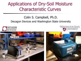
Applications of Dry-Soil Moisture Characteristic Curves Colin S. Campbell, Ph.D. Decagon Devices and Washington State University
Introduction • Decagon Devices • Started in 1983 supplying instrumentation for measuring water potential • Goal • Develop robust instrumentation to take accurate data AND fit within a budget • Vision • In the future, measuring and modeling the natural environment will require more high quality, innovative, and inexpensive solutions
Background • Colin Campbell • Ph.D. in Soil Physics, 2000, Texas A&M University • Vice President of Research, Development, and Engineering, Decagon Devices, Inc. • Adjunct Associate Professor of Environmental Biophysics, Washington State University • Current research • Insights into plant water use through combining soil moisture and morphology
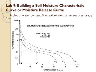
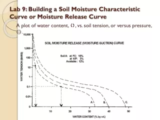
Soil Moisture Characteristic Curve (SMCC) • Moisture release curve, water retention function, pF curve, moisture sorption isotherm • Relationship between water content and water potential (water activity, suction, pF, chi)
Generating SMCC • Measuring water content is easy • Gravimetric analysis (oven drying) • Measuring water potential is difficult • No single instrument can make accurate measurements from wet to dry
Wet end instruments (liquid equilibrium) Wind-Schindler (HyProp) Pressure chamber Tensiometers
Dry end instruments (vapor equilibrium) Chilled mirror dew-point hygrometer Thermocouple psychrometers Relative humidity (hr) and water potential (Ψ) related by the Kelvin equation: R is universal gas constant Mw is molecular mass of water T is temperature
Dry end SMCC • Historically very difficult to obtain • Campbell and Shiozawa (1992) cited over 70 times and data used many by many authors • Introduction of WP4, WP4T, WP4C made dry end SMCC more accessible • Aquasorp/VSA instruments are the next step
VSA (Vapor Sorption Analyzer) • Generates dry end SMCC • Fully automated • Drying and wetting (hysteresis loop)
VSA limitation • Limitation: only works drier than -7 MPa (95% relative humidity)
Fan Optical Sensor Mirror Infrared Sensor Sample VSA (how it works) • Dynamic mode • Wet (~99% rh) or dry (~0%rh) air flows across sample • Flow stops and water activity/water potential and mass (water content) measured • Extreme resolution (> 200 points) • < 48 hours for wetting and drying loop (often < 10 hours) Dry Air Wet Air Precision Balance
Fan Optical Sensor Mirror Infrared Sensor Sample VSA (how it works) • Static mode • Humidity of chamber controlled at pre-determined level • Mass measured over time until no longer changing • Less resolution • Sorption kinetics • Sorption/desorption of other gases is possible Dry Air Wet Air Precision Balance
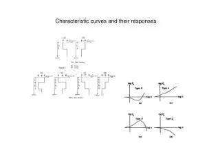
Slope of semi-log plot • Logarithm of water potential vs. water content • Plot becomes straight line in dry (VSA) region • Slope of plot contains much useful information
pF and Chi (Χ)Condon (2006), Orchiston, 1953 • pF = log (Ψ) where Ψ has units of cm of water • Common measure in Europe and in geotechnical engineering community • Takes log of number with units (mathematical mistake) • Increases with decreasing moisture (not intuitive) • Χ = -ln[-ln(aw)] where aw is water activity (relative humidity) • Mathematically correct, decreases with decreasing moisture
Slope of semi-log plot • Adsorption leg of semi-log plot extends through -1000 MPa at 0 water content • pF 7.0, Chi = -2.00 • aw = 0.0006, relative humidity = 0.06% • Slopes highly variable by soil type
What can you do with VSA data?Specific Surface Area (SSA) • BET model (Brunauer et al. 1938, Likos and Lu 2002) • Physically based model for isotherms (SMCCs) Water activity Water content offset slope Xm is water content when soil covered with monolayer of water
What can you do with VSA data?Specific Surface Area (SSA) • Slope of Chi plot (Condon 2006) SSA= f*S*a S is slope of Chi plot (g/g) a is monolayer coverage (3500 m2 g-1) f is factor of 1.84
What can you do with VSA data?Specific Surface Area (SSA) • Tuller and Or (2005) • General scaling model for SSA from SWCC • Mixed results in literature • Resurreccion (2011) • Used slope of log water potential vs. water content function for SSA
What can you do with VSA data?Specific Surface Area (SSA) Which SSA measure is the best? Still much research to be done!
What can you do with VSA data?Adsorbed cation type • Smectite exchanged to achieve homoionic state • Fundamentally different isotherms
What can you do with VSA data?CEC (cation exchange capacity) • “Intrinsic Isotherm” approach • Water content normalized by dividing by CEC of soil • All isotherms converge • Maybe inverse relationship could be used to predict CEC? • More research needed! Lu and Likos
What can you do with VSA data?Soil clay content (clay activity) • Resurreccion (2011) • Used slope of log water potential vs. water content function for SSA • Decagon internal research • Used slope of chi plot
What can you do with VSA data?Gas movement in soil • Simulations of water vapor transport for pesticide volatilization (Chen et al., 2000) • Remediation of Volatile Organic Carbon compounds (Batterman et al., 1995)
What can you do with VSA data?Swelling potential (expansiveness) • McKeen (1992) showed that the slope of pF vs. water content is related to soil swelling potential
What can you do with VSA data?Swelling potential (expansiveness) • Other possible swelling potential indicators • Breadth and area of hysteresis loop? • Monolayer coverage and heat of hydration from BET analysis? • Equilibrium water content at specific relative humidity • Sorption rate constants derived from step change in relative humidity (possible with new VSA) • MUCH more research needs to be done!
What can you do with VSA data?Unexplained results • Bentonite SMCCs (isotherms) • Desorption curve independent of starting water activity • Adsorption curve totally dependent on starting water activity
Take-home points • Aquasorp/VSA data useful for • Specific surface area • CEC • Clay activity • Swelling potential • Modeling of gas transport in soil • Sorption kinetics (not even explored yet) • We have not even begun to understand the usefulness of dry end SMCC/isotherms
References Batterman, S.A., A. Kulshrethsa, and H.Y. Chang. 1995. Hydrocarbonvapourtransport in lowmoisturesoils . Environmental Science and Technology 29: 171-180 Brunauer, S., P. H. Emmett, and E. Teller. 1938. Adsorption of gases in multi-molecular layers. J. Am. Chem. Soc. 60:309-319. Chen, D., D.E. Rolston, and P. Moldrup. 2000. Coupling diazinon volatilization and water evaporation in unsaturated soils: I. Water transport, Soil Science 165: 681-689 Condon, J. B. 2006. Surface Area and Porosity Determination by Physisorption: Measurements and Theory. Elsevier, Amsterdam. Likos, W. J. and N. Lu. 2002. Water vapor sorption behavior of smectite-kaolinite mixtures. Clays and Clay Minerals 50: 553-561. Orchiston, H. D. 1953. Adsorption of water vapor: I. Soils at 25 C. Soil Sci. 73:453-465 Resurrecction, A. C., P. Moldrup, M. Tuller, T.P.A. Ferre, K. Kawamoto, T. Komatsu, L. W. de Jonge. Relationship between specific surface area and the dry end of the water retention curve for soils with varying clay and organic carbon contents. Water Resources Research 47, W06522 Tuller, M. and D. Or. 2005. Water films and scaling of soil characteristic curves at low water contents. Water Resources Research 41, W09403.
Appendix: wet end measurements • Range can be extended further into wet end • Start with saturated sample and dry down • Can only get drying leg of hysteresis loop • VSA can’t wet back up past about -10 MPa using vapor equilibration