Download
1 / 37
440 likes | 889 Vues
Gause ’ s and Park ’ s competition experiments Lotka-Volterra Competition equations dN i /dt = r i N i ({K i – N i – S a ij N j }/K i ) Summation is over j from 1 to n , excluding i

E N D
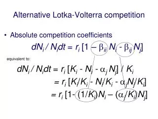
Gause’s and Park’s competition experiments Lotka-Volterra Competition equations dNi /dt = ri Ni ({Ki – Ni – S aij Nj }/Ki ) Summation is over j from 1 to n, excluding i Ni* = Ki – S aij NjAssumptions: linear response to crowding both within and between species, no lag in response to change in density, r, K, a constant Competition coefficients aij, i is species affected and j is the species having the effect Solving for zero isoclines, resultant vector analyses Four cases, depending on K/a’s compared to K’s Sp. 1 wins, sp. 2 wins, either/or, or coexistence
Four Possible Cases of Competition Under the Lotka–Volterra Competition Equations______________________________________________________________________ Species 1 can contain Species 1 cannot contain Species 2 (K2/a21 < K1) Species 2 (K2/a21 > K1) ______________________________________________________________________Species 2 can contain Case 3: Either species Case 2: Species 2Species 1 (K1/a12 < K2) can win always wins______________________________________________________________________Species 2 cannot contain Case 1: Species 1 Case 4: Neither speciesSpecies 1 (K1/a12 > K2) always wins can contain the other; stable coexistence______________________________________________________________________ Vito Volterra Alfred J. Lotka
Saddle Point Point Attractor
Lotka-Volterra Competition Equations for 3 species: dN1 /dt = r1 N1 ({K1 – N1 – a12 N2 – a13 N3 }/K1) dN2 /dt = r2 N2 ({K2 – N2 – a21 N1 – a23 N3 }/K2) dN3 /dt = r3 N3 ({K3 – N3 – a31 N1 – a32 N2 }/K2) Isoclines: (K1 – N1 – a12 N2 – a13 N3 )/K1 = 0when N1 = K1 – a12 N2 – a13 N3 (K2 – N2 – a21 N1 – a23 N3 )/K2 = 0when N2 = K2 – a21 N1 – a23 N3 (K3 – N3 – a31 N1 – a32 N2 )/K3 = 0when N3 = K3 – a31 N1 – a32 N2 Lotka-Volterra Competition Equations for n species (i = 1, n): dNi /dt = riNi ({Ki – Ni – S aij Nj}/Ki) Ni* = Ki – S aij Nj where the summation is over j from 1 to n, excluding iDiffuse CompetitionS aij Nj
Mutualism Equations (pp. 234-235, Chapter 11) dN1 /dt = r1 N1 ({X1 – N1 + a12 N2 }/X1)dN2 /dt = r2 N2 ({X2 – N2 + a21 N1 }/X2) (X1 – N1 + a12 N2 )/X1 = 0when N1 = X1 + a12 N2 (X2 – N2 + a21 N1 )/X2 = 0when N2 = X2 + a21 N1 If X1 and X2 are positive and a12 and a21 are chosen so that isoclines cross, a stable joint equilibrium exists. Intraspecific self damping must be stronger than interspecific positive mutualistic effects.
Hutchinsonian ratios among short wing Accipiter hawks Thomas W. Schoener
The ecological niche, function of a species in the community Resource utilization functions (RUFs) Competitive communities in equilibrium with their resources Hutchinson’s n-dimensional hypervolume concept Euclidean distances in n- space (Greek mathematician, 300 BC) Fundamental versus Realized Niches
Ecological Niche = sum total of adaptations of an organismic unit How does the organism conform to its particular environment? Resource Utilization Functions = RUFs Niche breadth and niche overlap
n-Dimensional Hypervolume Model Fitness density Hutchinson’s Fundamental and Realized Niches G. E. Hutchinson
One Dimension: Distance between two points along a line: simply subtract smaller value from larger one x2-x1 = d Two Dimensions: Score position of each point on the first and second dimensions. Subtract smaller from larger on both dimensions. d1=x2-x1 d2=y2-y1 Square these differences, sum them and take the square root. This is the distance between the points in 2D: sqrt (d12+ d22) = d Three Dimensions —> n-dimensions: follow this same protocol summing over all dimensions i = 1, n: sqrt Sdi2 = d Euclid
Euclidean distance between two species in n-space n-dimensional hypervolume djk = sqrt [S (pij - pik)2] where j and k represent species j and species k the pij and pik’s represent the proportional utilization or electivities of resource state i used by species j and species k, respectively and the summation is from i = 1 to n . n is the number of resource dimensions n Euclid i = 1
Niche Dimensionality 1 D = ~ 2 Neighbors 2 D = ~ 6 Neighbors 3 D = ~ 12 Neighbors 4 D = ~ 16 Neighbors 5 D = ~ 30 Neighbors NN = 2D + (D2 - D)Diffuse CompetitiondNi/dt = riNi(Ki -Ni-ij Nj)dNi/dt = 0 when Ni =Ki-ij Nj
Niche Breadth Jack of all trades is a master of noneMacArthur & Levin’s Theory of Limiting Similarity Robert H. MacArthur Richard Levins Specialists are favored when resources are very different
Niche Breadth Jack of all trades is a master of none MacArthur & Levin’s Theory of Limiting Similarity Robert H. MacArthur Richard Levins Generalists are favored when resources are more similar
Within-phenotype versus between-phenotype components of niche width
Complementarity of Niche Dimensions, page 276 Anolis Thomas W. Schoener
Resource matrices of utilization coefficients Niche dynamics Niche dimensionality and diffuse competition Complementarity of niche dimensions Niche Breadth: Specialization versus generalization. Similar resources favor specialists, Different resources favor generalists Periodic table of lizard niches (many dimensions) Thermoregulatory axis: thermoconformers —> thermoregulators
Experimental Ecology Controls Manipulation Replicates Pseudoreplication Rocky Intertidal Space Limited System Paine’s Pisaster removal experiment Connell: Balanus and Chthamalus Menge’s Leptasterias and Pisaster experiment Dunham’s Big Bend saxicolous lizards Brown’s Seed Predation experiments Simberloff-Wilson’s defaunation experiment
R. T. Paine (1966)
Joseph Connell (1961)
Bruce Menge (1972)
Menge 1972 Bruce Menge
Grapevine Hills, Big Bend National Park Sceloporusmerriami and Urosaurusornatus Six rocky outcrops: 2 controls, 2 Sceloporus removal plots and 2 Urosaurus removal areas. ======================================================== 4 year study: 2 wet and 2 dry: insect abundances Monitored density, feeding success, growth rates, body weights, survival, lipid levels Urosaurus removal did not effect Sceloporus density No effects during wet years (insect food plentiful) Insects scarce during dry years: Urosaurus growth and survival was higher on Sceloporus removal plots Arthur Dunham