Decoupling PDEs: Explore Shock Profiles and State Space Dynamics
Using initial conditions and PDEs to decouple systems, analyze the behavior of shock profiles and state space dynamics over time. Discover how pulses move and the evolution of curves in 2D state space scenarios. Explore different kinds of waves like rarefractions, compressions, and simple waves. Understand Ahat and P-Systems, Euler's Full Gas Equations, and solutions to Maxwell's Equations through eigenvectors and Lie brackets.

Decoupling PDEs: Explore Shock Profiles and State Space Dynamics
E N D
Presentation Transcript
Update By Rob Chase and Pat Dragon Supervised by Robin Young
Given initial conditions and a system of PDEs, what happens? The decoupled case can be modeled (u,v)t+(u+v,u-v)x=0 (u,v)t+(u,v)x=0 Decoupling is equivalent to finding the eigensystem
Recall Shock Profiles u-x Initial Conditions: u = exp[-x^2] As time goes on, burgur’s (backward) flux function the pulse will move to the right (left).
Recall Phase Plane t-x Initial Conditions: u = exp[x] The straight lines represent level curves.
Recall State Space u-v Initial Conditions: u = exp[-x^2] v = exp[-x^2] The Curve is a parametric function of x with one bell curve superimposed on the other as shock profiles.
State Space 2D t=.1 As the two pulses diverge (one going left, the other right), the curve billows out.
State Space 2D t=.5 The curve in state space continues to change…
State Space 2D t=1.1 t-x (u) t-x (v) The characteristics begin to overdefine the function…
State Space 2D t=2 The shock “eats” information (whatever u,v symbolize) and very little is left over at the end. The horizontal and vertical lines are where the shock profile has become overdefined.
Kinds of Waves Constant Solutions 2D surfaces
Simple Waves One Dimensional image in state space
The Riemann Problem Given an initial state and a final state, can simple waves connect them? Rarefractions Compressions Shocks The curves found by integrating the eigenvectors represent a locus of states connected to the initial conditions.
Ahat-System: If U=(u,v,w) and Ahat is a 2x2 matrix Ut+Ahat(U)Ux=0 wt+f(w)wx=0
P-System: The shock tube is immersed in water of constant temperature ut + a*v^(-g)*x = 0 a, g constants vt - ux = 0 0 p’(v) -1 0 +/- c = Sqrt[-p’(v)] (c,1) (-c,1)
Euler’s Full Gas Equations(holy grail) The Elastic String Ut+Vx=0 Vt+T(U)x=0 pt + (pv)x = 0 (pv)t + (pv^2+P)x = 0 Et + (v(E+P))x = 0 Plane Solutions to Maxwell’s Equations
Lie Brackets of Eigenvectors Definition: [X,Y] = D[Y]X-D[X]Y Frobeneous: If [X,Y] = 0 Then the vectors define a surface
To do… Find Eigensystems Integrate Eigenvectors Lie Bracket the Eigenvectors