Group Symmetry Models
Group Symmetry Models. Appendix A of: Symmetry and Lattice Conditional Independence in a Multivariate Normal Distribution. by Andersson & Madsen. Presented by Shaun Deaton.

Group Symmetry Models
E N D
Presentation Transcript
Group Symmetry Models Appendix A of: Symmetry and Lattice Conditional Independence in a Multivariate Normal Distribution. by Andersson& Madsen. Presented by Shaun Deaton
Let a random vector in ℝ6 with a multivariate normal distribution N(0, Σ), having zero mean and covariance matrix . dof=21
Introduce symmetry constraints; i.e. invertible linear transformations mapping the observation vector space ℝ6 into itself. Consider for Example the sample vectors having components paired as shown below. This can be likened to measurements across three controlled populations or to measurements on three attributes of an individual (There are many variations, that can be chosen for the situation. ). In this case: Let x1, x3, and x5 all represent the same observable, only each is restricted to a distinct object. Similarly, the remaining variables x2, x4, and x6 represent the same observable property possessed by each object. Run experiment and collect data by measuring the two observable properties of each object. Obtaining at least N ≥ I samples from ℝ6 to ensure MLE existence. Perform usual multivariate analysis to obtain empirical covariance . Object A Object B Object C
Now introducing symmetry constraints from G1, a set of symmetries, requires the following block form for the covariance matrix. Where Id is the identity transformation and swap is a permutation interchanging A & B. dof=12 Let G1 = { Id, swap(A,B) } B A C Rewriting the covariance matrix in block form using 2x2 symmetric positive definite matrices gives the following: Where generally:
Another set of symmetry constraints that could be imposed on the analysis are given by G2. There are the two symmetries from before, plus four others, which can be seen as all symmetries of an equilateral triangle. Let G2 = { Id, swap(A,B), swap(A,C), swap(B,C), (A,B)(B,C)=CAB, (A,C)(B,C)=BCA } dof=6 A B C Rewriting this covariance matrix using the 2x2 symmetric matrices as before, gives the following: Where generally:
Note that symmetries can manifest in many different contexts: (algebraic symmetry by permuting variables) x1 + x2 + x3 + x4 + x5 + x6 Is symmetric under all actions of G2. x1 x2 + x3 x4 + x5 x6 Is symmetric under all actions of G1. Same as swap(1,3)swap(2,4). Has more symmetries than this… Then there is … x12x2 + x32x4 + x52x6
The measured samples vectors can be arranged into an N x 6 matrix in this example; generally an N x I matrix for I variables per sample. Let this data matrix be denoted by ; with a double arrow for being a vector of vectors. This notation is used for a convenient symbolizing when one wants to refer to all of the vector samples , or just one of the I x 1 vectors . More explicitly: Under the multivariate normal model, with zero mean, the empirical covariance matrix is calculated by: is an (I x N) x (N x I) = I x I matrix.
Hypothesis Testing works in the same fashion; by looking at the ratio of maximized likelihood functions under each hypothesis. (Then infer rejection via a chi-square or more generalized distribution.) Where I in exp is from the trace of the I×I identity matrix, obtained from . Which also defines the MLE sigma for the larger dof (degree-of-freedom); ‘big’ hypothesis. For the smaller dof (‘null’) hypothesis, the maximization gives . Where , and the new N x 6 matrix , must be such that . At least this is what is being tested; whether the covariance of the data has this symmetry or not.
Testing the data for this covariance symmetry is achieved by operating on the sample covariance matrix , transforming it into a new matrix to use in the likelihood ratio test. The NxI data matrix is not transformed into a new ‘symmetrized’ data set . Although, there is such a relationship, it is more complicated and involves extra calculation, rather than just ‘symmetrizing’ the sample covariance. Now can view the null hypothesis, that the covariance matrix has some group symmetry, at the data level of sample vectors; which comes down to saying that any and all samples may be transformed into new samples giving the same statistical information as far as the model is concerned. This idea is illustrated in the next slide, where a sample vector is assumed to be transformed by some invertible linear transformation . The possibilities for this transformation are generated from those belonging to the group G.
The linear transformation , must remain unchanged by all symmetries under consideration, and all symmetries must form a group. Now, consider the following where is an invertible linear transformation and is one of the symmetry operations like the swap illustrated below*; then looking at the variable used by the exp() function in N(0, Σ): Letting , then obtain . Showing that the transformation of a sample vector by a symmetry does not change the shape of the underlying distribution. Which is another way to view the situation, that is, the probability distribution over the sample space has symmetry; i.e. like the geometric shapes above for the distributions graphical form and like the polynomials above for the functional form of the distribution; if there is one. *E.g. a swap(A,B) symmetry applied to a general matrix of 2x2 block matrices.
There is a valid invertible transformation for every symmetry restriction. Giving |G| total number of transformed sample data, including the original data due to the identity transformation always being present. Since essentially everything has the identity symmetry; just do nothing. Still require to be a invariant (i.e. unchanged) by all symmetry actions. But, it is not, instead a group (used same as symmetry) action gives the following: . This shows that an element of the same form results, so the affect of applying all group actions is to permute the set of all transformed versions of the measured data. That is the |G| in total, N x 6 data matrices are swapped around in their entirety. The only group action that fixes is the identity action, so its asymmetric, and so must increase its symmetry to the whole group.
Creating symmetric objects. Given any non-symmetric shape, i.e. has only invariance under identity, action, like… Turn it into a shape that has a non-trivial symmetry; here overlapping six copies of the shape, each rotated by a multiple of 600, generates the new shape. Having the rotational symmetriesof a regular hexagon, denoted by C6. From this shape another can be generated by copying & reflecting about the vertical line shown. Now, all symmetries of a hexagon are possessed by this final shape, denoted by D6 ; i.e. all ways it can be flipped & rotated while afterwards being unchanged; of which there are 12 ways. The C6 & D6 symbols are just standard group names specifying a collection of symmetries.
Likewise a similar idea is applied to the empirical covariance matrix, increasing the number of matrices to a total of |G|, by applying all symmetry operations. The ‘overlapping’ in this case is replaced by matrix addition, which is then averaged by dividing by |G|. -The formula for the transformation is given by: -Where the resulting matrix has the following G-invariant property: . This MLE is then used for a likelihood ratio test to determine if the assumed symmetry structure is present in the objects under experiment.
Let H be a subgroup of G. Then the covariance matrix can be symmetrized under each group structure and tested. Since a larger group means more symmetry restriction there will be a decrease in the dof of the model, giving an inverse relationship between subgroups of groups and sub-hypothesis of hypothesis. H = HId , here the identity just gives the usual empirical covariance. H0 = HH , matrix symmetry under H. H00 = HG , matrix symmetry under G. More to come … ?
Definition: A group is a set with a closed binary operation, defined on it, denoted by ‘*’, such that the following holds: (where closed means the operation does not give elements outside of the set.) Associative Law– (a*b)*c = a*(b*c) Identity Law– There is a unique element Id, where Id*g = g*Id = g, for all elements g in the group. Inverse Law– Every group element has a unique inverse; i.e. given any element g, can find an element h where g*h = h*g = Id. Additionally, a group representation is a mapping of the group G into the group of invertible linear transformations GL(V), on some n-D vector space V. In our case V is the I-D sample space ℝI, and G is mapped to a special subgroup of GL(V), composed of all orthogonal matrices O(V); i.e. from the matrix view those where the transpose of a matrix is its inverse. This is the reason for the transpose operator for some of the group operations, it’s the inverse under the orthogonal representation. Back
Note: This slide is an aside from the previous material, it looks more into applying the symmetrization to the underlying data, not the covariance. About calculating the symmetrized covariance matrix straight from the data; (which is not the way to go, especially for efficiency). The action on the sample vectors turns into a similar action on the N x I data matrix: The |G| diagonal terms give the correct symmetrization, just need a change of variables to put the transposition in the right place using the following to transform the initial sample vectors; gives the usual conjugation form. Although the |G|2 - |G| extra, off diagonal terms, do not cancel. When summed pair-wise with their transpose related term, they form |G|(|G|- 1)/2 symmetric matrices. These “cross-conjugation” terms are interesting, I am still going to look into the problem from this perspective, though will not spend too much time on it.