Affine Invariant Triangulation
Affine Invariant Triangulation. Ashish Myles. Overview. Goals/Motivation Delaunay Delaunay-based affine-invariant method Barycentric coordinates-based method. Goal and Motivation. Compute a “nice” triangulation of a point set P Connectivity should be affine invariant Application:

Affine Invariant Triangulation
E N D
Presentation Transcript
Affine Invariant Triangulation Ashish Myles
Overview • Goals/Motivation • Delaunay • Delaunay-based affine-invariant method • Barycentric coordinates-based method
Goal and Motivation • Compute a “nice” triangulation of a point set P • Connectivity should be affine invariant • Application: • 1-D b-spline knots (domain) – affine invariant • 2-D simplex spline knots need to be triangulated; desire affine invariance
Delaunay – Strengths • Simple and intuitive criterion (circle-based) – makes proofs easy • Invariant under rotations, reflections and uniform scaling • Globally Local Delaunay Global Delaunay • Implies uniqueness (up to degeneracy) • Guaranteed convergence of edge-flips • Objective function: maximize minimum angle • Convexity-check built-in
Delaunay Weaknesses • Not general-affine invariant
Affine-Invariant Delaunay • Apply principal components analysis • Rescale to make the principal components equal • Compute Delaunay triangulation • Rescale back to original data set • Demo
Affine-Invariant Delaunay • C = • C = U D UT, U orthogonal, D diagonal • A = D½ UT • Run Delaunay on A-1(P–M), M = (x, x) to get T’ • T = A T’ + M is the final triangulation
Affine-Invariant Delaunay • Advantages: • Same as regular Delaunay + affine-invariance • Disadvantages: • Point-insertion global transformation change • Concept of locally “good” tainted by global transformation
Barycentric-Based Approach ua + vb + wc = p (1/w)p – (u/w)a – (v/w)b = c –(v/u)b + (1/u)p – (w/u)c = a –(u/v)a + (1/v)p – (w/v)c = b • Goodness: • g(ab) = min(u/v, v/u) 1 • g(cd) = min(-w, -1/w) 1
Barycentric-Based Approach • Geometric intuition • g(edge) = min(dist)/max(dist) = min(area)/max(area) • Choose edge with max goodness (good if closer to 1)
Barycentric-Based Approach • Advantages • Point insertion does not automatically invalidate all edge choices • Automatic convexity check: g(ab) < g(cd)
Barycentric-Based Approach • Disadvantages • No proofs for convergence for edge flips • Conjecture: converge to a local maximum • No proofs for uniqueness • Globally local good does not mean globally good • Conjecture: not always unique? • No obviously good choice for objective function • Max min goodness? • Max average goodness?