Real-Time Pulse Detection System for Low Signal Environments
300 likes | 445 Vues
This system aims for accurate pulse detection in low signal settings, providing frequency and strength output, while rejecting noise spikes. Using DSP, the algorithm works with an 80MHz processor to achieve less than 25% false identifications. The detection process involves a two-for-one FFT approach, weighted average computation, and pulse differentiation, ensuring efficiency and reliability in real-time pulse identification. System testing involves signal manipulation with various SNR levels, validating its robustness.

Real-Time Pulse Detection System for Low Signal Environments
E N D
Presentation Transcript
DSP Pulse Detection System Patrick Auchter Mark Paul
Project Goals • Detection of pulses in a low signal to noise ratio environment • Requires a fast algorithm • Rejection of noise spikes • Less than 25% of identifications are false identifications • Output the strength and frequency of pulse
System Overview • DSP samples at 44.1 kHz • 64 samples are collected every 1.45 ms • Input levels are -1 to 1 Volt • The processor is 80 MHz • Compiled code is loaded into the DSP through a parallel port using Code Composer Studio • The serial port is used to output binary data such as the pulse magnitude
Two-for-One FFT • A complex FFT is performed to take the FFT of two real sequences at once • The two output sequences are separated through the following equations
Assembly Buffer Setup 0 1 2 3 4 5 1020 1021 1022 1023 ↕ • The formulas for separating X(f) and Y(f) are
FFT Routine • First the input data is bit-reversed • Then a Radix-2 FFT is performed 000 → 000 001 → 100 010 → 010 011 → 110 100 → 001 101 → 101 110 → 011 111 → 111
Applying FFTs to Input Data • The DSP collects 64 new input samples every time the Two-for-One FFT is performed • The two buffers of FFT data are separated by 32 samples x 1 y x 2 y
Cost of the FFT • An N-point FFT costs N*log2(N) multiply-accumulates • After performing the two-for-one FFT, separating the two sequences requires 2*N additions • Using the two-for-one FFT saves us N*log2(N) multiply-accumulates, but adds 2*N additions • Calculating the magnitude of the frequency data requires 2*N multiplications and N additions
Detection Algorithm • A weighted average of the last 70 maximums in the frequency domain is calculated • Each maximum is multiplied by its corresponding weight and added to the total • The weighted average is the total divided by the sum of the weights • For a length 70 buffer, the sum of the weights is 42 • Computing the weighted average costs L multiply-accumulates, where L is the buffer length
Detection of Strong Pulses • The weighted average is used to determine if there is a pulse in the current window of FFT data • If the maximum is over 30 times the weighted average, it is definitely a pulse • Otherwise, we can check for a weak pulse
Detection of Weak Pulses • All of the FFT data over 3.4 times the weighted average is stored so that the width of the pulse can be determined • We check to make sure that the frequency difference of the points is less than or equal to 3 points or 258 Hz • We also check to make sure that the maximum in the current FFT data and the maximum in the previous FFT data are at the same frequency
Updating the Weighted Average • The following guidelines are used to determine when to update the weighted average • If the maximum is less than 3.4 times the weighted average, it is added to the maximum buffer and the weighted average is recalculated • Otherwise, the maximum is not added, since the maximum is either a noise spike or a pulse • Adding these maximums would undesirably increase the weighted average, making it more difficult to detect weak pulses
Challenges • Zero-padding and the two-for-one FFT • Designing a fast, efficient algorithm to process the data in real time • Testing all the data we collected and looking for abnormalities and weak pulses to test the system’s performance
Testing • Various signal-to-noise ratio signals were used to test and improve the system • Signals with odd noises were also tested to ensure that the noises did not cause false detections • We manipulated the following parameters to obtain the best results • FFT size • Length of the maximum buffer • Factors for determining strong and weak pulses • Length of the frequency window to analyze
Various SNR Signals 9.11 dB 3.09 dB -2.92 dB -6.44 dB
Effect of Decreasing Signal to Noise Ratio 9.11 dB 3.09 dB -2.92 dB -6.44 dB
Successes • The system consistently detects most of the audible pulses • When the pulse power is half the noise power, we detect the pulse 85 percent of the time • Less than 10% of the detections are noise • We do not use all of the clock cycles every pass, so additional processing of the data could be done if needed