Download

1 / 54
540 likes | 564 Vues
Learn to prepare, run, and create dynamic optimization applications using Object-Oriented API in Risk Solver Platform. Understand mathematical modeling, decision variables, objective functions, and constraints. Step-by-step guide to transforming problems into models and solving them efficiently.

E N D
Spreadsheet-Based Decision Support Systems Chapter 19: Solver Re-Visited Prof. Name name@email.com Position (123) 456-7890 University Name
Overview • 19.1 Introduction • 19.2 Review of Chapter 8 • 19.3 Object – Oriented API in Risk Solver Platform • 19.4 Application • 19.5 Summary
Introduction • Preparing an optimization problem to be solved by the Solver • Preparing and running the Risk Solver Platform using Object–Oriented API • Creating a dynamic optimization application using Object – Oriented API
Review of Chapter 8 • Understanding the problem • Preparing the spreadsheet • Solving the Model
Review of Chapter 8 • In Chapter 8 we described how to transform a problem into a mathematical model and then use the Risk Solver Platform to solve it. • We will review the main parts of a mathematical model and the Solver preparation steps. • There are important steps which take place in the Excel spreadsheet before the Solver is used. • Reading and Interpreting the Problem • Preparing the Spreadsheet • Solving the Model and Reviewing the Results
Understanding the Problem • Mathematical models transform a word problem into a set of equations that clearly define the values you are seeking given the limitations of the problem. • There are three main parts of a mathematical model. • Decision variables • Objective function • Constraints
Decision Variables • Decision variables are variables that are assigned to a quantity or response that you must determine in the problem. • They can be defined as negative, non-negative, or unrestricted variables. • An unrestricted variable can be either negative or non-negative. • These variables are used to represent all other relationships in the model, including the objective function and constraints.
Objective Function • The objective function is an equation that states the goal, or objective, of the model. • Objective functions are either maximized or minimized. • Most applications involve maximizing profit or minimizing cost.
Constraints • The constraints are the limitations of the problem. • In most realistic problems there are certain limitations, or constraints, which we must satisfy. • Constraints can be a limited amount of resources, labor, or requirements for a particular demand. • These constraints are also written as equations in terms of the decision variables.
Applying a Mathematical Model • We saw some examples in Chapter 8 which involved production of different parts. • The amount to produce of each part was considered the decision variables. • Maximizing profit (given certain costs and revenues for each part) was the objective function. • There were also constraints which limited the resources needed for each part and stated a minimum demand that had to be met.
Preparing the Spreadsheet • We must translate and clearly define each part of our model in the spreadsheet. • The Solver will then interpret our model according to how we have declared the decision variables, objective function, and constraints in the spreadsheet. • We use referencing and formulas to mathematically represent the model in the spreadsheet cells.
Entering Decision Variables • To enter the decision variables, we list them in individual cells with an empty cell next to each one. • The Solver will place values in these cells for each decision variable as it solves the model. • All other equations (for the objective function and constraints) will reference these cells.
Entering Objective Function • To enter the objective function, we place our objective function equation in a cell with an adjacent description. • This equation should be entered as a formula which references the decision variable cells. • As the Solver changes the decision variable values in the decision variable cells, the objective function value will automatically be updated.
Entering Constraints • To enter the constraints we list the equations separately with a description next to each constraint. • The most important part of setting up the constraint table is expressing the left side of our equations as formulas. • As each constraint is in terms of the decision variables, all of these formulas must be in terms of the decision variable cells that Solver uses. • These equations should reference the decision variable cells so that as the Solver places values in these cells the constraint values will automatically be calculated. • Another important consideration when laying out the constraints in preparation for Solver is that the RHS (right-hand side) values of each constraint should be in individual cells to the right of these equations. • We should also place all inequality signs in their own cells.
Naming the Ranges • Another advantageous way to keep our constraints organized as we use the Solver is to name our cells. • Using the methods discussed in Chapter 3, we can name the ranges decision variables and the cell which holds the objective function equation. • We can also name ranges of constraint equations which are in a similar category of constraints or which have similar inequality signs. • This makes inserting these model parts into the Solver easier when using both Excel and VBA code .
Solver Example from Chapter 8 • A company produces six different types of products. They want to schedule their production to determine how much of each product type should be produced in order to maximize their profits. This is known as the Product Mix problem. • Production of each product type requires labor and raw materials; but the company is limited by the amount of resources available. • There is also a limited demand for each product, and no more than this demand per product type can be produced. Input tables for the necessary resources and the demand are given.
Step 1 • Decision Variables: The amount produced of each product type. • x1, x2, x3, x4, x5, x6 • Objective Function: Maximize Profit. • z = p1*x1 + p2*x2 + p3*x3 + p4*x4 + p5*x5 + p6*x6 • Constraints: There are two resource constraints: labor, l, and raw material, r. • Labor Constraint: • l1*x1 + l 2*x2 + l 3*x3 + l4*x4 + l 5*x5 + l 6*x6 <= available labor = 4500 • Raw Material Constraint • r1*x1 + r 2*x2 + r 3*x3 + r 4*x4 + r 5*x5 + r 6*x6 <= available raw material = 1600 • There is also a constraint that all demand, D, must be met, and no extra amount can be produced. • Demand Constraint: • xi <= Di for i = 1 to 6
Figure 19.1 • The Spreadsheet layout for the Product Mix
Figure 19.2 • Risk Solver Task Pane: • Set the Objective to the location of the objective function formula. • Set the Variables to the empty decision variable cells named “PMDecVar”. • The Constraints show the left and right sides of the constraint equations with the corresponding inequalities. • The labor and raw material constraints are listed as Normal constraints. • Demand constraints are listed as the Bound constraints since they set an upper limit on the value that the decision variables can take. • Set the Assume Non-Negative property of the model to true.
Figure 19.3 • The Results of the Solver are shown. • All constraints are met.
Object-Oriented API in Risk Solver Platform • Building a Problem Using Object-Oriented API • Identifying the Solver Engine and Setting its Parameters • Running the Solver • Accessing Optimization Results
Object-Oriented API in Risk Solver Platform • Use object-oriented API to create a problem initially, and then add the decision variables, objective function, and constraints. From Tools > References list on the VBE select Risk Solver Platform xx Type Library. • Use VBA code to manipulate Engine parameters, and optimize the problem using VBA commands. • Access the results of the optimization, such as, objective function value, optimal solution, dual variables, etc.
Building a Problem Using Object-Oriented API • We start by creating an instance of the Problemobject. The Problemobject represents the whole optimization problem. We declare this object variable using the Dim statement as follows: • Dim MyProb As New RSP.Problem • Set the SolverType property of the Solver object to Maximize or Minimize to specify whether the optimization problem should be maximized or minimized. • The values that the SolverType property takes are: • Solver_Type_FindFeas (find a feasible solution) • Solver_Type_Maximize (maximize) • Solver_Type_Minimize (minimize) • Solver_Type_Simulate (simulate)
Adding New Decision Variables • To add new decision variables to MyProb, we create a Variable object, initialize the object, set its properties, and then add this object to the Variable collection of the problem object. • Use the Init method to specify the range which contains the decision variables. • Use the Variables.Add method to add the decision variables to the problem object. Dim MyVar As New Variable MyVar.Init Range("DecisionVariables") MyVar.NonNegative MyProb.Variables.Add MyVar Set MyVar = Nothing
Adding the Objective Function • To add the objective function to MyProb, we create a Function object, initialize this object, set its properties, add it to the Functions collection of the problem, and finally set its value to nothing. • Use the Init method to specify the range of the objective function. • Use the FunctionType property to identify the type of the function that is being added to the problem. • This property takes the value Function_Type_Objective for the objective function, and Function_Type_Constraint for normal constraints. DimMyObjAs NewRSP.Function MyObj.Init Range("ProdObjFunc") MyObj.FunctionType = Function_Type_Objective MyProb.Functions.AddMyObj Set MyObj = Nothing
Adding Constraints • Use a ForNext loop to add each individual constraint. • Create an array of Functions objects using the Dim statement. • The size of this array is set to the total number of constraints. • Use the Init method specifies the range which contains a constraint equation. • The Relation method allows us to specify the relation (<=, =, or >=) and the RHS value of the constraints.. • The constants Cons_Rel_EQ (=), Cons_Rel_GE (>=) or Cons_Rel_LE (<=) are used to specify the relation. • The Add method is used to add each individual constraint to the end of the Function collection of the problem object.
Adding Constraints (cont’d) Dim MyConstraints(NumCons) As New RSP.Function For i = 1 To NumCons MyConstraints (i).Init Range("A1").Offset(i - 1, 0) MyConstraints (i).Relation Cons_Rel_GE, Range("B1").Offset(i - 1, 0).Value MyConstraints (i).FunctionType = Function_Type_Constraint MyProb.Functions.Add MyConstraints (i) Set MyConstraints (i) = Nothing Next • The Remove method allows us to delete constraints from the problem formulation. • The only parameter this function takes is the index of the constraint that will be removed. The following statement removes the last constraint of MyProb. • MyProb.Functions.Remove NumCons
Identifying Solver Engine and Parameters • Prior to solving an optimization problem, we should specify the appropriate Solver Engine to use. • For an optimization problem, the Engine object represents the LP/Quadratic, StandardEvolutionary or the GRGNonlinear solver depending on the type of the problem we are solving. • When the Solver.Optimize method is then called, this engine will run. • If the problem we are working with is a linear program, we will select the LP/Quadratic Solver using: • MyProb.Engine = MyProb.Engines("Standard LP/Quadratic") • Prior to modifying Solver Engine parameters you should reset all the parameters to their default value by using the ParamReset method. • MyProb.Engine.ParamReset
Identifying Solver Engine and Parameters • There are a large number of problem parameters for a particular Solver Engine. • Use the Name property to identify the name and the index of a parameter of interest. Use this index to access and modify the corresponding parameter. Fori = 0 ToMyProb.Engine.Params.Count - 1 IfMyProb.Engine.Params(i).Name = "Iterations" Then MyProb.Engine.Params(i).Value = 100 EndIf Nexti MyProb.Engine.Params(“AssumeNonneg”).Value = True
Running the Solver • Use Solver.Optimize() method to run the Solver. • This method’s only argument, Solve_Type,takes two values: • Solve_Type_Analyze to perform a model analysis without actually solving, • Solve_Type_Solve to solve the optimization problem. MyProb.Solver.Optimize (Solve_Type) • The OptimizeStatus property of the Solver object returns an integer value classifying the result of the optimization. • The values 0, 1, or 2 signify a successful run in which a solution has been found. • The value 4 implies that there was no convergence • The value 5 implies that no feasible solution could be found.
Running the Solver (cont’d) Dim result As Integer result = MyProb.Solver.OptimizeStatus If result = 5 Then MsgBox “Your problem was infeasible. Please modify your model.” EndIf • Solver.Optimize is the only command needed to run the Solver. • If we have already set up the Solver in the spreadsheet or in some initial part of the VBA code, at execution time, we need to write only the Solver.Optimize command.
Accessing Optimization Results • We can access the results of the optimization by using the Value property of Variable object, or FinalValue, DualValue and Slack properties of the Function object. • VBA is also used to automatically generate the solution reports listed in the Report drop-down menu of the Ribbon. • The Size property of VarDecision object identifies the total number of the decision variables in a problem. For i = 0 To MyProb.VarDecision.Size - 1 MsgBox MyProb.VarDecision.Value(i) Next i
Accessing Optimization Results (cont’d) • The Count property of the Functions object identifies the total number of functions in the Problem object. • MsgBox MyProb.Functions(MyProb.Functions.Count - 1).Value(0) • To print the dual variables for problem constraints, we would write: For i = 0 To MyProb.Functions.Count - 2 MsgBox MyProb.Functions(i).DualValue(0) Next i • If we decide to generate the reports, then we need to set the value of Bypass Solver Reports engine parameter to False. • After the Solver has finished running, we can access the reports using the following statement. • Solver.Report ReportName
Accessing Optimization Results (cont’d) • ReportName is one of the following strings “Answer”, “Feasibility”, “Linearity”, “Limits”, “Population”, “Sensitivity”, “Scaling”, and “Solution”. • The Report method generates a report in the form of an Excel worksheet and inserts it into the active workbook.
Other Solver Methods • The Init method instantiates a problem using a named model or worksheet. • This method creates the variable and function objects using an optimization problem already defined in the worksheet. • The Save method is used to save model specifications in a cell range, or as a text string model name. • The Load method is used to load model specifications. • Format is one of the parameters required by this method. This parameter is a constant which takes one of the following two values: • File_Format_XLStd or File_Format_XLPSI.
Example Code 1 • Use this VBA code to: • Initiate a problem using a model already defined in an existing Excel worksheet. • Save problem parameters. • Solve the problem. • Display the objective function value found from the optimization. Sub Init_Save_Prob_Methods() Dim prob As New RSP.Problem prob.Init Worksheets("Prob_Setup") prob.Save Worksheets("Prob_Save").Range(“A1”) prob.Solver.Optimize MsgBox prob.Functions(prob.Functions.Count - 1).Value(0) EndSub
Example Code 2 • Using the following lines of code you can load the model you already saved, optimize the problem, and display the corresponding objective function value. Sub Load_Prob_Method() Dim prob As New RSP.Problem, Param As Range Set Param = Worksheets("Prob_Save").Range(Range(“A1”),Range(“A1”). End(xlDown)) prob.Load Param, File_Format_XLStd prob.Solver.Optimize MsgBox prob.Functions(prob.Functions.Count - 1).Value(0) EndSub
Application • Dynamic Production Problem
Description • We consider a production problem in which we are trying to determine how much to produce of different items in order to maximize profit. • Each item has a given weight, space requirement, profit value, quota to satisfy, and limit on production. • Each item must meet its quota but be less than its limit. • There is also a total weight requirement and space requirement for shipping which will limit the production.
Dynamic Solver • We want this production problem to be dynamic. • We want the user to decide how many items to consider in the problem and to provide the input for each item. • We limit these dynamic options to five possible items and prepare the spreadsheet for the maximum number possible. • To make this problem dynamic, we will develop a user interface.
Figure 19.5 • The Parameters form asks the users for the number of decision variables.
Figure 19.6 • The Input form is dynamic in that it allows the users to enter input values for the number of items they specified in the Parameters form.
Initial Code • We will have a main procedure associated with the Solve Dynamic Problem button called SetParameters. In this procedure, we • Initialize our range variables • Call the ClearPrev procedure • Show the users the first form (the second form will be shown from the first form code). • Redefine our dynamic ranges by using the values for the number of decision variables (NumDV) and the number of constraints (NumCons) identified in the code of the first form. • Call the SolveProb procedure procedure.
Figure 19.7 • We show the variable declarations and code for the SetParameters procedure and a ClearPrev procedure.
Figure 19.8 • Parameters Form code.
Figure 19.9 • Input Form code.
Figure 19.10 • After initializing the text box arrays, it is easy to set these default values simply by looping through each array
Figure 19.11 • This part of SolveProb procedure creates a problem instance and adds the corresponding decision variables, constraints and objective function.
Figure 19.12 • This part of SolveProb procedure selects an engine, sets engine parameters, solves the problem, and calls the ViewResults procedure.