Biometrical genetics

1. Biometrical genetics Pak C Sham The University of Hong Kong Manuel AR Ferreira Queensland Institute for Medical Research 23rd International Workshop on Methodology of Twin and Family Studies 2nd March, 2010

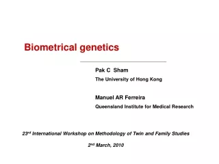
2. ADE Model for twin data 1/0.25 MZ/DZ 1/0.5 E1 D1 A1 A2 D2 E2 e c a a c e Y1 Y2

3. Biometrical Genetics

4. Outline 1. Basic molecular genetics 2. Components of genetic model 3. Biometrical properties for single locus 4. Introduction to linkage analysis

5. 1. Basic molecular genetics

6. DNA A DNA molecule is a linear backbone of alternating sugar residues and phosphate groups Attached to carbon atom 1’ of each sugar is a nitrogenous base: A, C, G or T Complementarity: A always pairs with T, likewise C with G A gene is a segment of DNA which is translated to a peptide chain nucleotide

7. Human genome 23 chromosome pairs 22 autosomes, X,Y ~ 33,000,000,000 base pairs ~ 25,000 translated “genes” Other functional sequences non-translated RNA binding sites for regulatory molecules

8. DNA sequence variation (polymorphisms) Microsatellites >100,000 Many alleles, eg. (CA)n repeats, very informative, easily automated Single nucleotide polymorphims (SNPs) 11,883,685 (build 128, 03 Mar ‘08) Most with 2 alleles (up to 4), not very informative, easily automated A Copy Number polymorphisms Large-scale insertions / deletions B A

9. Fertilization and mitotic cell division 22 + 1 2 (22 + 1) 2 (22 + 1) 2 (22 + 1) ♂ ♁ ♂ A - A - A - ♁ B - ♂ ♁ ♁ ♂ Mitosis B - B - chr1 A - A - A - - A A - - A ♁ ♁ ♂ B - B - B - - B B - - B A - - A - A B - - B - B chr1 G1 phase S phase M phase Haploid gametes Diploid zygote 1 cell Diploid somatic cells

10. Meiosis / Gamete formation 22 + 1 22 + 1 A - NR (♂) B - A - - A chr1 2 (22 + 1) 2 (22 + 1) B - - B - A ♁ Meiosis R chr1 (♂) (♁) ♂ ♁ - B A - A - - A - A chr1 B - B - - B - B A - R chr1 chr1 chr1 chr1 (♁) A - - A B - chr1 Diploid gamete precursor cell B - - B - A chr1 NR - B Haploid gamete precursors chr1 Hap. gametes

11. 2. Components of genetic model

12. A. Transmission model Mendel’s law of segregation Mother (A3A4) Segregation (Meiosis) Gametes A3(½) A4(½) A1(½) A1A3(¼) A1A4(¼) Father (A1A2) Offspring A2(½) A2A4(¼) A2A3(¼) Note: 50:50 segregation can be distorted (“meiotic drive”)

13. A. Transmission model: two unlinked loci Phase: A1B1 / A2B2 Locus B (B1B2) Segregation (Meiosis) B2(½) B1(½) A1(½) A1B1(1/4) A1B2(1/4) Locus A (A1A2) Gametes A2(½) A2B1(1/4) A2B2(1/4)

14. A. Transmission model: two linked loci Phase: A1B1 / A2B2 Locus B (B1B2) Segregation (Meiosis) B2(½) B1(½) A1(½) A1B1((1-)/2) A1B2(/2) Locus A (A1A2) Gametes A2(½) A2B1(/2) A2B2((1-)/2)  : Recombination fraction, between 0 (complete linkage) and 1/2 (free recombination)

15. B: Population model Frequencies aa AA Aa aa AA Aa AA AA AA Aa aa AA Genotype frequencies: AA: P Aa: Q aa: R Allele frequencies: A: P+Q/2 a: R+Q/2

16. B: Population model Hardy-Weinberg Equilibrium (Hardy GH, 1908; Weinberg W, 1908) Random mating Offspring genotypic distribution

17. B: Population model Hardy-Weinberg Equilibrium (Hardy GH, 1908; Weinberg W, 1908) Offspring genotype frequencies Offspring allele frequencies

18. B. Population model Panmixia (Random union of gametes) Maternal allele A (p) a (q) P (AA) = p2 P (Aa) = 2pq A (p) AA (p2) Aa (pq) Paternal allele P (aa) = q2 a (q) aa (q2) aA (qp) Deviations from HWE Assortative mating Imbreeding Population stratification Selection

19. C. Phenotype model Classical Mendelian (Single-gene) traits Dominant trait - AA, Aa1 - aa0 Huntington’s disease (CAG)n repeat, huntingtin gene Recessive trait - AA 1 - aa, Aa0 Cystic fibrosis 3 bp deletion exon 10 CFTR gene

20. 1 Gene  3 Genotypes  3 Phenotypes 2 Genes  9 Genotypes  5 Phenotypes 3 Genes  27 Genotypes  7 Phenotypes 4 Genes  81 Genotypes  9 Phenotypes C. Phenotype model Polygenic model Central Limit Theorem  Normal Distribution

21. AA Aa aa C. Phenotype model Quantitative traits e.g. cholesterol levels

22. D. Phenotype model Aa Fisher’s model for single quantitative trait locus (QTL) P(X) aa AA X +a d Genotypic effects – a p2 2pq Genotype frequencies q2 Assumption: Effect of allele independent of parental origin (Aa = aA) Violated in genomic imprinting

23. 3. Biometrical properties of single locus

24. Biometrical model for single biallelic QTL 1. Contribution of the QTL to the Mean (X) Genotypes Aa aa AA a d -a Effect, x p2 2pq q2 Frequencies, f(x) Mean (X) = m = a(p2) + d(2pq) – a(q2) = (p-q)a + 2pqd Note: If everyone in population has genotype aa then population mean = -a  change in mean due to A = ((p-q)a + 2pqd) – (-a)= 2p(a+qd)

25. Biometrical model for single biallelic QTL 2. Contribution of the QTL to the Variance (X) Genotypes Aa aa AA a d -a Effect, x p2 2pq q2 Frequencies, f(x) Var (X) = (a-m)2p2 + (d-m)22pq + (-a-m)2q2 = 2pq(a+(q-p)d)2 + (2pqd)2 = VQTL Broad-sense heritability of X at this locus = VQTL/ V Total

26. Biometrical model for single biallelic QTL 2. Partitioning of QTL variance: additive component Maternal allele A (p) a (q) Average A (p) a d pa+qd Paternal allele a (q) -a pd-qa d pd-qa Average pa+qd (p-q)a + 2pqd Variance due to a single allele =p(q(d+a)-2pqd)2+q(p(d-a)-2pqd)2 =pq(a+(q-p)d)2 For both alleles, additive variance = 2pq(a+(q-p)d)2

27. Biometrical model for single biallelic QTL 2. Partitioning of QTL variance: dominance component Genotype Effect Additive effect AA (p2) 2(pa+qd) a Aa (2pq) (pa+qd)+(pd-qa) d aa (q2) -a 2(pd-qa) Dominance variance due to QTL =p2(a-2(pa+qd))2 +2pq(d-(pa+qd+pd-qa))2 +q2(-a-2(pd-qa) = (2pqd)2

28. Biometrical model for single biallelic QTL a 0 Genotypic effects -a aa AA aa AA aa AA Aa Aa Aa Additive Dominant Recessive Var (X) = Regression Variance + Residual Variance = Additive Variance + Dominance Variance = VAQTL+ VDQTL

29. Statistical definition of dominance is scale dependent +4 +4 +0.7 +0.4 log (x) aa AA aa AA Aa Aa No departure from additivity Significant departure from additivity

30. Practical H:\ferreira\biometric\sgene.exe

31. Practical Aim Visualize graphically how allele frequencies, genetic effects, dominance, etc, influence trait mean and variance Ex1 a=0, d=0, p=0.4, Residual Variance = 0.04, Scale = 2. Vary a from 0 to 1. Ex2 a=1, d=0, p=0.4, Residual Variance = 0.04, Scale = 2. Vary d from -1 to 1. Ex3 a=1, d=0, p=0.4, Residual Variance = 0.04, Scale = 2. Vary p from 0 to 1. Look at scatter-plot, histogram and variance components.

32. Some conclusions • Additive genetic variance depends on allele frequency p & additive genetic value a as well as dominance deviation d • Additive genetic variance typically greater than dominance variance

33. Biometrical model for single biallelic QTL 1. Contribution of the QTL to the Mean (X) 2. Contribution of the QTL to the Variance (X) 3. Contribution of the QTL to the Covariance (X,Y)

34. Biometrical model for single biallelic QTL 3. Contribution of the QTL to the Cov (X,Y) (a-m) Aa aa (-a-m) (d-m) AA (a-m)2 (a-m) AA (d-m) (a-m) (d-m) (d-m)2 Aa aa (-a-m)2 (-a-m) (-a-m) (d-m) (-a-m) (a-m)

35. Biometrical model for single biallelic QTL 3A. Contribution of the QTL to the Cov (X,Y) – MZ twins (a-m) Aa aa (-a-m) (d-m) AA p2 (a-m)2 (a-m) AA (d-m) (a-m) (d-m) (d-m)2 Aa 0 2pq aa (-a-m)2 (-a-m) (-a-m) (d-m) (-a-m) q2 0 (a-m) 0 Cov(X,Y) = (a-m)2p2 + (d-m)22pq + (-a-m)2q2 = VAQTL+ VDQTL =2pq[a+(q-p)d]2 + (2pqd)2

36. Biometrical model for single biallelic QTL 3B. Contribution of the QTL to the Cov (X,Y) – Parent-Offspring (a-m) Aa aa (-a-m) (d-m) AA p3 (a-m)2 (a-m) AA (d-m) (a-m) (d-m) (d-m)2 Aa p2q pq aa (-a-m)2 (-a-m) (-a-m) (d-m) (-a-m) q3 0 (a-m) pq2

37. e.g. given an AAfather, an AAoffspring can come from either AAx AAor AAx Aaparental mating types AAx AA will occur p2× p2 = p4 and have AA offspring Prob()=1 AAx Aa will occur p2× 2pq = 2p3q and have AA offspring Prob()=0.5 and have Aa offspring Prob()=0.5 Therefore, P(AA father & AAoffspring) = p4 + p3q = p3(p+q) = p3

38. Biometrical model for single biallelic QTL 3B. Contribution of the QTL to the Cov (X,Y) – Parent-Offspring (a-m) Aa aa (-a-m) (d-m) AA p3 (a-m)2 (a-m) AA (d-m) (a-m) (d-m) (d-m)2 Aa p2q pq aa (-a-m)2 (-a-m) (-a-m) (d-m) (-a-m) q3 0 (a-m) pq2 Cov (X,Y) = (a-m)2p3 + … + (-a-m)2q3 = ½VAQTL =pq[a+(q-p)d]2

39. Biometrical model for single biallelic QTL 3C. Contribution of the QTL to the Cov (X,Y) – Unrelated individuals (a-m) Aa aa (-a-m) (d-m) AA p4 (a-m)2 (a-m) AA (d-m) (a-m) (d-m) (d-m)2 Aa 2p3q 4p2q2 aa (-a-m)2 (-a-m) (-a-m) (d-m) (-a-m) q4 p2q2 (a-m) 2pq3 Cov (X,Y) = (a-m)2p4 + … + (-a-m)2q4 = 0

40. Biometrical model for single biallelic QTL 3D. Contribution of the QTL to the Cov (X,Y) – DZ twins and full sibs ¼ genome ¼ genome ¼ genome ¼ genome # identical alleles inherited from parents 2 1 (father) 0 1 (mother) ¼ (2 alleles) + ½ (1 allele) + ¼ (0 alleles) Unrelateds MZ twins P-O Cov (X,Y) = ¼ Cov(MZ) + ½ Cov(P-O) + ¼ Cov(Unrel) = ¼(VAQTL+VDQTL) + ½ (½ VAQTL) + ¼ (0) = ½ VAQTL + ¼VDQTL

41. Summary so far…

42. Biometrical model predicts contribution of a QTL to the mean, variance and covariances of a trait Association analysis = a(p-q) + 2pqd Mean (X) Linkage analysis = VAQTL+ VDQTL Var (X) = VAQTL+ VDQTL Cov (MZ) On average! = ½VAQTL+ ¼VDQTL Cov (DZ) For a sib-pair, do the two sibs have 0, 1 or 2 alleles in common? 0, 1/2 or 1 0 or 1 IBD estimation / Linkage

43. 4. Introduction to Linkage Analysis

44. For a heritable trait... Linkage: localize region of the genome where a QTL that regulates the trait is likely to be harboured Family-specific phenomenon: Affected individuals in a family share the same ancestral predisposing DNA segment at a given QTL Association: identify a QTL that regulates the trait Population-specific phenomenon: Affected individuals in a population share the same ancestral predisposing DNA segment at a given QTL

45. Linkage Analysis: Parametric vs. Nonparametric Gene Chromosome Recombination Genetic factors M Q A Mode of inheritance Dominant trait 1 - AA, Aa 0 - aa Correlation D Phe C E Environmental factors Adapted from Weiss & Terwilliger 2000

46. Approach Parametric: genotypes marker locus & genotypes trait locus (latter inferred from phenotype according to a specific disease model) Parameter of interest: θbetween marker and trait loci Nonparametric: genotypes marker locus & phenotype If a trait locus truly regulates the expression of a phenotype, then two relatives with similar phenotypes should have similar genotypes at a marker in the vicinity of the trait locus, and vice-versa. Interest: correlation between phenotypic similarity and marker genotypic similarity No need to specify mode of inheritance, allele frequencies, etc...

47. Phenotypic similarity between relatives Squared trait differences Squared trait sums Trait cross-product Trait variance-covariance matrix Affection concordance T2 T1

48. Genotypic similarity between relatives IBSAlleles shared Identical By State “look the same”, may have the same DNA sequence but they are not necessarily derived from a known common ancestor M3 M1 M2 M3 Q3 Q1 Q2 Q4 IBDAlleles shared Identical By Descent are a copy of the same ancestor allele M1 M2 M3 M3 Q1 Q2 Q3 Q4 IBD IBS M1 M3 M1 M3 2 1 Q1 Q4 Q1 Q3 0 0 1 0 1 Inheritance vector (M)

49. Genotypic similarity between relatives - Inheritance vector (M) Number of alleles shared IBD Proportion of alleles shared IBD - M2 M3 M1 M3 0 0 0 1 1 0 Q2 Q4 Q1 Q3 M1 M3 M1 M3 0 0 1 0 0.5 1 Q1 Q4 Q1 Q3 M1 M3 M1 M3 0 0 0 0 2 1 Q1 Q3 Q1 Q3

50. Genotypic similarity between relatives - D A B C 22n