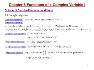
Complex Algebra: Differentiation and Integration of Functions
Explore differentiation and integration of complex functions, roots of equations, logarithms, de Moivre’s theorem, and application in differential equations. Understand principles of real and complex variable differentiation and integration.

Complex Algebra: Differentiation and Integration of Functions
E N D
Presentation Transcript
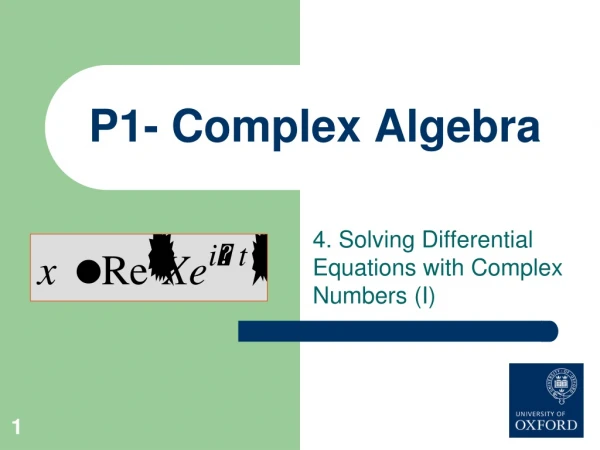
P1- Complex Algebra 3. Further functions, Differentiation and Integration of Complex Functions
Im eiθ Re Summary of previous lecture • The roots to equations of the form lie equispaced on a circle on an Argand diagram. • There are n roots. • The first root has argument θ/nand the others follow by 2π/n.
Summary cont. • The natural logarithm of a complex number is multi-valuedin the complex domain • Solutions to equations of complex variables trace loci (lines, curves, circles, ellipses) in the complex plane.
Summary cont. • de Moivre’s theorem
Summary cont. • Complex functions render manipulation of products of trigonometric and exponential functions simpler. Substituting the following expressions can be particularly useful:
Contents 3.1 Differentiation of complex functions wrt a real variable 3.2 Differentiation of complex functions wrt a complex variable 3.3 Integration of complex functions 3.4 Homogeneous linear 2nd order ordinary differential equations 3.5 Higher order homogenous linear ordinary differential equations
3.1Differentiation of complex functions wrt. real variables • The derivative of a function fwith respect to a real variable x is defined as: • if and only if the function is continuous in the range x to x+δx.
Differentiation wrt. real variables cont. • If a complex function f only depends on iand one real variable, we can treat i as a constant and differentiate thatfunction with respect to the real variable as usual. • All the usual rules of differentiation apply in that case: where c is a constant and f and g are both functions of a complex variable that only depends oniand θ.
Differentiation wrt. real variables cont. • e.g. By writing cosθas a sum of complex exponentials, find its derivative with respect toθ.
Differentiation wrt. real variables cont. • e.g.Find the derivative of with respect to θ.
Differentiation wrt. real variables cont. • Alternatively
3.2 Differentiation of complex functions wrt. complex variables • The derivative of a function f of a complex variable z is defined as: if and only if the function is analytic in the range z to z+δz (i.e. if it can be expressed as a Taylor series at any point).
Differentiation wrt. complex variables cont. • The Cauchy-Riemann equations can be used to determine whether a complex function is analytic. However, this is well beyond the scope of this course. • If complex functions are analytic (and you will be told whether they are), then their derivative with respect to the complex variable z exists and all the known rules of differentiation apply.
Differentiation wrt. complex variables cont. e.g. Determine the derivative of sinh(z) with respect to z, given that it is analytic in the complex domain.
3.3 Integration of complex functions • Integration of functions of complex variables follows the same rules as for real variables. • We can exploit this property to integrate products of exponential and trigonometric functions.
Integration of complex functions cont. • e.g. find
3.4 Homogeneous linear 2nd order ordinary differential equations • e.g. Consider a mass mounted on a spring and a damper. We assume that the spring and the damper are linear, that the spring provides a force proportional to its extension and the damper a force proportional to the rate of extension.
Homogeneous linear 2nd order ODEs cont. • The equation of motion of the mass is • If we select a trial solution then
Homogeneous linear 2nd order ODEs cont. • Substituting these into the equation of motion gives • which has roots
Homogeneous linear 2nd order ODEs cont. • These roots will be real or complex depending on the relative magnitude of λ and 4km if damping is high, roots are real if damping is low, roots are complex
x xo t Homogeneous linear 2nd order ODEs cont. • For the case where there will be 2 real roots and thus the solution is The system is said to be OVERDAMPED
x xo t Homogeneous linear 2nd order ODEs cont. • For the case where there will be a repeated real roots and thus the solution is The system is said to be CRITICALLY DAMPED
Homogeneous linear 2nd order ODEs cont. • For the solutions in s are • If we make the substitutions and we have
Homogeneous linear 2nd order ODEs cont. • which gives the following solution
Homogeneous linear 2nd order ODEs cont. • thus the solution in this case will be an exponentially decaying sinusoid Over damped (c= 1.5) Critically damped (c= 1.0) Under damped (c = 0.2)
Homogeneous linear 2nd order ODEs cont. • To complete the solution it is necessary to find the constants A1 and A2. • These will in general be complex and are determined by the initial conditions, i.e. the known values of x and at t = 0 .
Homogeneous linear 2nd order ODEs cont. • Let us assume that the initial position of the mass is x = 0 and its initial velocity = v. The solution has the general form: • Setting t = 0 we get
Homogeneous linear 2nd order ODEs cont. • Differentiating x with respect to t gives • Setting t = 0 gives
Homogeneous linear 2nd order ODEs cont. • Solving the two simultaneous equations for A1 and A2 gives
Homogeneous linear 2nd order ODEs cont. • Substituting those back into the expression for x
Homogeneous linear 2nd order ODEs cont. • In trigonometric form
Homogeneous linear 2nd order ODEs cont. • Simplifying leads to the solution for the differential equation • ωnis known as the undamped natural frequency, • cas the damping constant and • ωn√(1-c2) as the damped natural frequency.
3.5 Higher order homogeneous linear ordinary differential equations • The same approach can be used to find the solution to linear differential equations with constant coefficients of higher order also. • The general method is to substitute a trial solution of the form , giving
Higher order differential equations cont. • On cancelling the exponentials, we obtain the auxiliary polynomial • Each root of the polynomial, s1, s2, s3,… sn, produces a solution to the ODE.
Higher order differential equations cont. • If two (or more) roots are repeated, then we have to substitute a modified solution function of the form • The solution to the original differential equation is then sum of all the n separate solutions: