Complex number : Complex algebra: Complex conjugation:
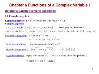
Chapter 6 Functions of a Complex Variable I. October 3 Cauchy-Riemann conditions 6.1 Complex algebra. Complex number : Complex algebra: Complex conjugation:. Polar representation:. Modulus (magnitude):. Argument (phase):. Functions of a complex variable:

Complex number : Complex algebra: Complex conjugation:
E N D
Presentation Transcript
Chapter 6 Functions of a Complex Variable I October 3 Cauchy-Riemann conditions 6.1 Complex algebra Complex number: Complex algebra: Complex conjugation: Polar representation: Modulus (magnitude): Argument (phase):
Functions of a complex variable: All elementary functions of real variables may be extended into the complex plane. A complex function can be resolved into its real part and imaginary part: Multi-valued functions and branch cuts: To remove the ambiguity, we can limit all phases to (-p,p). q = -p is the branch cut. lnz with n = 0 is the principle value. We can let z move on 2 Riemann sheets so that is single valued everywhere.
6.2 Cauchy-Riemann conditions Analytic functions: If f (z) is differentiable at z = z0 and within the neighborhood of z=z0, f (z) is said to be analytic at z = z0. A function that is analytic in the whole complex plane is called an entire function. Cauchy-Riemann conditions for differentiability In order to let f be differentiable, f '(z) must be the same in any direction of Dz. Particularly , it is necessary that Cauchy-Riemann conditions
Conversely, if the Cauchy-Riemann conditions are satisfied, f (z) is differentiable: More about Cauchy-Riemann conditions: 1) It is a very strong restraint to functions of a complex variable. 2) 3) 4)
Reading: General search for Cauchy-Riemann conditions: Our Cauchy-Riemann conditions were derived by requiring f '(z) be the same when z changes along x or y directions. How about other directions? Here I do a general search for the conditions of differentiability.
Read: Chapter 6: 1-2 Homework: 6.1.7,6.1.17,6.2.1,6.2.8 Due: October 14
October 7 Cauchy’s theorem 6.3 Cauchy’s integral theorem Contour integral: Cauchy’s integral theorem: If f (z) is analytic in a simply connected region R, [and f ′(z) is continuous throughout this region, ] then for any closed path C in R, the contour integral of f (z) around C is zero: Proof using Stokes’ theorem:
Cauchy-Goursat proof: The continuity of f '(z) is not necessary. Corollary: An open contour integral for an analytic function is independent of the path, if there is no singular points between the paths. z2 z2 z1 z1 Contour deformation theorem: A contour of a complex integral can be arbitrarily deformed through an analytic region without changing the integral. 1) It applies to both open and closed contours. 2) One can even split closed contours. Proof: Deform the contour bit by bit. “nails” C2 C1 “rubber bands” Examples: 1) Cauchy’s integral theorem. (Let the contour shrink to a point.) 2) Cauchy’s integral formula. (Let the contour shrink to a small circle.) C2 C2 C3 C1 C1
6.4 Cauchy’s integral formula Cauchy’s integral formula:If f (z) is analytic within and on a closed contour C, then for any point z0 within C, L1 C C0 L2 z0 Can directly use the contour deformation theorem.
Derivativesof f (z): Corollary: If a function is analytic, then its derivatives of all orders exist. Corollary: If a function is analytic, then it can be expanded in Taylor series. Cauchy’s inequality: If is analytic and bounded, then Liouville’s theorem: If a function is analytic and bounded in the entire complex plane, then this function is a constant. Fundamental theorem of algebra: has n roots. Suppose P(z) has no roots, then 1/P(z) is analytic and bounded as Then P(z) is constant. That is nonsense. Therefore P(z) has at least one root we can divide out.
Morera’s theorem:If f (z) is continuous and for every closed contour within a simply connected region, then f (z) is analytic in this region.
Read: Chapter 6: 3-4 Homework: 6.4.1,6.4.3,6.4.4 Due: October 14
October 10 Analytic continuation 6.5 Laurent expansion Taylor expansion for functions of a complex variable: Expanding an analytic function f (z) about z = z0, where z1 is the nearest singular point. z
Schwarz’s reflection principle:If f (z) is 1) analytic over a region including the real axis, and 2) real when z is real, then Examples: most of the elementary functions.
Analytic continuation: Suppose f (z) is analytic around z = z0, we can expand it about z = z0 in a Taylor series: This series converges inside a circle with a radius of convergence , where a0 is the nearest singularity from z = z0. We can also expand f (z) about another point z = z1 within the circle R0: . In general, the new circle has a radius of convergence and contains points not within the first circle. a0 R0 z0 z1 R1 a1 Consequences: 1) f (z) can be analytically continued over the complex plane, excluding singularities. 2) If f (z) is analytic, its values at one region determines its values everywhere.
Read: Chapter 6: 5 Homework: 6.5.2,6.5.5 Due: October 21
October 12 Laurent expansion 6.5 Laurent expansion Problem: Expanding a function f (z) that is analytic in an annular region (between r and R). L2 L1 C is any contour that encloses z0 and lies between r and R (deformation theorem).
Laurent expansion: • Singular points of the integrand. For n < 0, the singular points are determined by f (z). For n ≥0, the singular points are determined by both f (z) and 1/(z'-z0)n+1. • If f (z) is analytic inside C, then the Laurent series reduces to a Taylor series: • Although an has a general contour integral form, In most times we need to use straight forward complex algebra to find an.
Laurent expansion: Examples Example 1: Expand about z0=1. Example 2: Expand about z0=i.
Read: Chapter 6: 5 Homework: 6.5.8,6.5.9,6.5.10 Due: October 21
October 17 Branch points and branch cuts 6.6 Singularities Poles: In a Laurent expansion then z0 is said to be a poleoforder n.A pole of order 1 is called a simple pole.A pole of infinite order (when expanded about z0) is called an essential singularity. The behavior of a function f (z) at infinity is defined using the behavior of f (1/t) at t = 0. Examples: sinz thus has an essential singularity at infinity.
Branch points and branch cuts: Branch point: A point z0 around which a function f (z) is discontinuous after going a small circuit. E.g., Branch cut: A curve drawn in the complex plane such that if a path is not allowed to cross this curve, a multi-valued function along the path will be single valued.Branch cuts are usually taken between pairs of branch points. E.g., for , the curve connects z=1 and z = can serve as a branch cut. Examples of branch points and branch cuts: If a is a rational number, then circling the branch point z = 0 q times will bring f (z) back to its original value. This branch point is said to be algebraic, and q is called the order of the branch point. If a is an irrational number, there will be no number of turns that can bring f (z) back to its original value. The branch point is said to be logarithmic.
A B A B We can choose a branch cut from z = -1 to z = 1 (or any curve connecting these two points). The function will be single-valued, because both points will be circled. Alternatively, we can choose a branch cut which connects each branch point to infinity. The function will be single-valued, because neither points will be circled. It is notable that these two choices result in different functions. E.g., if , then
Read: Chapter 6: 6 Homework: 6.6.1,6.6.2,6.6.3 Due: October 28
October 19 Mapping 6.7 Mapping y v Mapping: A complex function can be thought of as describing a mapping from the complex z-plane into the complex w-plane. In general, a point in the z-plane is mapped into a point in the w-plane. A curve in the z-plane is mapped into a curve in the w-plane. An area in the z-plane is mapped into an area in the w-plane. w1 z1 z0 w0 x u z w Examples of mapping: Translation: Rotation:
Inversion: In Cartesian coordinates: A straight line is mapped into a circle:
6.8 Conformal mapping Conformal mapping: The function w(z) is said to be conformal at z0 if it preserves the angle between any two curves through z0. If w(z) is analytic and w'(z0)0, thenw(z) is conformal at z0. Proof: Since w(z) is analytic and w'(z0)0, we can expand w(z) around z = z0 in a Taylor series: • At any point where w(z) is conformal, the mapping consists of a rotation and a dilation. • The local amount of rotation and dilation varies from point to point. Therefore a straight line is usually mapped into a curve. • A curvilinear orthogonal coordinate system is mapped to another curvilinear orthogonal coordinate system .
What happens if w'(z0) = 0? Suppose w (n)(z0) is the first non-vanishing derivative at z0. This means that at z = z0 the angle between any two curves is magnified by a factor n and then rotated by b.
Read: Chapter 6: 7-8 Homework: 6.7.1,6.7.2,6.8.1 Due: October 28