ISQA 459/559 Advanced Forecasting
270 likes | 570 Vues
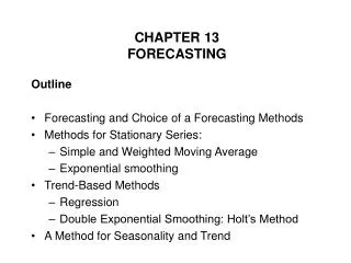
ISQA 459/559 Advanced Forecasting. Mellie Pullman. Recall Forecast Error Measurements. MFE: mean forecast error MAD: mean absolute deviation. 30. Best Error Measurement (What it the problem with the MAD calculation as an error measurement for long histories?). 365 days Averaged ?.

ISQA 459/559 Advanced Forecasting
E N D
Presentation Transcript
ISQA 459/559Advanced Forecasting Mellie Pullman
Recall Forecast ErrorMeasurements • MFE: mean forecast error • MAD: mean absolute deviation 30
Best Error Measurement(What it the problem with the MAD calculation as an error measurement for long histories?) 365 days Averaged ?
Solution? • Smoothed MAD • Phi (j) is a smoothing parameter, which is set in advance. • It is important that we fix (set) phi BEFORE we try to find the best forecasting method. Why?
Phi • Phi controls the period of time over which we are evaluating forecast accuracy--the smaller the value of phi, the larger the number of historical periods that are considered in the measurement of the "average" forecast error. • What effect would changing phi have while you are trying to compare the accuracy of two different forecasting methods?
Quarter Year 1 Year 2 Year 3 Year 4 1 45 70 100 100 2 335 370 585 725 3 520 590 830 1160 4 100 170 285 215 Total 1000 1200 1800 2200 Average 250 300 450 550 Seasonal Index/Factor We estimate 2600 for Year 5 but need to know how many to make each quarter.
Quarter Year 1 Year 2 Year 3 Year 4 1 45/250 = 0.18 70 100 100 2 335 370 585 725 3 520 590 830 1160 4 100 170 285 215 Total 1000 1200 1800 2200 Average 250 300 450 550 45 250 Seasonal Index = = 0.18 Seasonal Index/Factor
Quarter Year 1 Year 2 Year 3 Year 4 1 45/250 = 0.18 70/300 = 0.23 100/450 = 0.22 100/550 = 0.18 2 335/250 = 1.34 370/300 = 1.23 585/450 = 1.30 725/550 = 1.32 3 520/250 = 2.08 590/300 = 1.97 830/450 = 1.84 1160/550 = 2.11 4 100/250 = 0.40 170/300 = 0.57 285/450 = 0.63 215/550 = 0.39 Quarter Average Seasonal Index 1 (0.18 + 0.23 + 0.22 + 0.18)/4 = 0.20 2 (1.34 + 1.23 + 1.30 + 1.32)/4 = 1.30 3 (2.08 + 1.97 + 1.84 + 2.11)/4 = 2.00 4 (0.40 + 0.57 + 0.63 + 0.39)/4 = 0.50 Seasonal Index/Factor
Quarter Year 1 Year 2 Year 3 Year 4 1 45/250 = 0.18 70/300 = 0.23 100/450 = 0.22 100/550 = 0.18 2 335/250 = 1.34 370/300 = 1.23 585/450 = 1.30 725/550 = 1.32 3 520/250 = 2.08 590/300 = 1.97 830/450 = 1.84 1160/550 = 2.11 4 100/250 = 0.40 170/300 = 0.57 285/450 = 0.63 215/550 = 0.39 Quarter Average Seasonal Index Forecast 1 (0.18 + 0.23 + 0.22 + 0.18)/4 = 0.20 650(0.20) = 130 2 (1.34 + 1.23 + 1.30 + 1.32)/4 = 1.30 650(1.30) = 845 3 (2.08 + 1.97 + 1.84 + 2.11)/4 = 2.00 650(2.00) = 1300 4 (0.40 + 0.57 + 0.63 + 0.39)/4 = 0.50 650(0.50) = 325 Seasonal Influences
Decomposition of Season & Trend • Decompose the data into components • Find seasonal component • Deseasonalize demand • Find Trend component • Forecast future values of each component • Project Trend component into future • Multiply trend component by seasonal component
Using Yearly Data to start? Using Monthly data to start? Options for Brewery Case that use regression and/or seasonal adjustment?
80 — 70 — 60 — 50 — 40 — 30 — Guest arrivals | | | | | | | | | | | | | | | 0 1 2 3 4 5 6 7 8 9 10 11 12 13 14 15 Week Trend-Adjusted Exponential Smoothing Actual room requests
80 — 70 — 60 — 50 — 40 — 30 — Guest Arrivals At = Dt + (1 - )(At-1 + Tt-1) Tt = (At - At-1) + (1 - )Tt-1 Guest arrivals | | | | | | | | | | | | | | | 0 1 2 3 4 5 6 7 8 9 10 11 12 13 14 15 Week Trend-Adjusted Exponential Smoothing
80 — 70 — 60 — 50 — 40 — 30 — Guest Arrivals At = Dt + (1 - )(At-1 + Tt-1) Tt = (At - At-1) + (1 - )Tt-1 Guest arrivals A0 = 28 g D1 = 27 g T0 = 3 g = 0.20 = 0.20 A1 = 0.2(27) + 0.80(28 + 3)= 30.2 T1 = 0.2(30.2 - 28) + 0.80(3)= 2.8 | | | | | | | | | | | | | | | 0 1 2 3 4 5 6 7 8 9 10 11 12 13 14 15 Week Trend-Adjusted Exponential Smoothing
80 — 70 — 60 — 50 — 40 — 30 — Guest Arrivals At = Dt + (1 - )(At-1 + Tt-1) Tt = (At - At-1) + (1 - )Tt-1 Guest arrivals A0 = 28 guests T0 = 3 guests = 0.20 = 0.20 A1 = 30.2 T1 = 2.8 Forecast2 = 30.2 + 2.8 = 33 | | | | | | | | | | | | | | | 0 1 2 3 4 5 6 7 8 9 10 11 12 13 14 15 Week Trend-Adjusted Exponential Smoothing
80 — 70 — 60 — 50 — 40 — 30 — Guest Arrivals At = Dt + (1 - )(At-1 + Tt-1) Tt = (At - At-1) + (1 - )Tt-1 Guest arrivals A1= 30.2 D2 = 44 T1 = 2.8 = 0.20 = 0.20 A2 = T2 = Forecast = | | | | | | | | | | | | | | | 0 1 2 3 4 5 6 7 8 9 10 11 12 13 14 15 Week Trend-Adjusted Exponential Smoothing
80 — 70 — 60 — 50 — 40 — 30 — Guest Arrivals At = Dt + (1 - )(At-1 + Tt-1) Tt = (At - At-1) + (1 - )Tt-1 Guest arrivals A1= 30.2 D2 = 44 T1 = 2.8 = 0.20 = 0.20 A2 = 35.2 T2 = 3.2 Forecast = 35.2 + 3.2 = 38.4 | | | | | | | | | | | | | | | 0 1 2 3 4 5 6 7 8 9 10 11 12 13 14 15 Week Trend-Adjusted Exponential Smoothing
80 — 70 — 60 — 50 — 40 — 30 — Guest arrivals | | | | | | | | | | | | | | | 0 1 2 3 4 5 6 7 8 9 10 11 12 13 14 15 Week Trend-Adjusted Exponential Smoothing Trend-adjusted forecast Actual guest arrivals
In Class Exercise • Amar = 300,000 cases; Tmar = +8,000 cases Dapr = 330,000 cases; a= 0.20 b=.10 • What are the forecasts for May and July?