Download
1 / 49
490 likes | 623 Vues
Characterization of the Earth’s Surface and Atmosphere from Thermal Imagery. Erich Hernandez-Baquero, Capt., USAF Ph.D. Dissertation Defense Advisor: Dr. John R. Schott 1 June 2000. Chester F. Carlson Center for Imaging Science Rochester Institute of Technology. Overview. Introduction

E N D
Characterization of the Earth’s Surface and Atmosphere from Thermal Imagery Erich Hernandez-Baquero, Capt., USAF Ph.D. Dissertation Defense Advisor: Dr. John R. Schott 1 June 2000 Chester F. Carlson Center for Imaging Science Rochester Institute of Technology
Overview • Introduction • Approach • Experimental Results • Conclusions • Questions & Discussion
Global Climate and Change • 1997-1998 El Niño • Record-setting • 2100 deaths • $33+ billion (U.S.D.) property damage • Global warming • Ozone depletion
The Problem • Target emission • Temperature • Emissivity • Atmospheric emission • Temperature profiles • Constituent concentration • Sensor • Spatial resolution • Spectral response • Detector thermal noise Challenge: infer information about the atmosphere and the surface directly from the hyperspectral cube Sensor: Atmosphere: Temperature Emissivity Target:
H2O CO2 O3 H2O H2O CO2 Thermal Spectrum
• Transmission • Upwelled radiance • Downwelled radiance Observed radiance Radiative Transfer Model Inputs • Atmospheric profiles • Weather conditions • Molecular spectroscopy • Surface temperature and emissivity Atmospheric Model Outputs
x1 y1 y2 x2 r1 v1 u1 y3 x3 r2 v2 u2 . . . . . . . . . rr ur vr xp yq CCA Path Diagram weights weights . . . loadings loadings
CCA (Cont.) The linear combinations are obtained from: Where e and f are the eigenvectors from: And r2 are the eigenvalues, which are the maximized correlations.
4 2 U 0 2 2 0 2 4 V CCA (cont.) Canonical Correlations in a Nutshell: • Linear combination maximizes correlation between U and V • U and V have unit variance • Several U-V pairs may be found with decreasing correlations • Linear combinations are orthogonal • No distinction between predictor and response variables n observations
CCA Example: Linnerud data Chins Situps Weight Waist Height Jumps
CCA Example Weight Chins Situps Waist Jumps Pulse
CCA Example chins & situps r jumps large waist low weight
CCA Implementation Canonical Variables MODTRAN CCA OR Radiosonde Correlations
Test & Verification MODTRAN Runs MODTRAN Inverse Model Radiosonde TES Ground Truth
CCA Implementation Canonical Variables MODTRAN CCA OR Radiosonde Correlations
Lake Mead, NV Date: 02 Dec 1998 Time: 1953 Zulu Altitude: 6.0 km Flight: 99-001-01F
Cold Springs, NV Date: 29 Sep 1999 Time: 1847 Zulu Altitude: 10.0 km Flight: 99-006-14F
CCA Implementation Canonical Variables MODTRAN CCA OR Radiosonde Correlations
CCA Implementation Canonical Variables MODTRAN CCA OR Radiosonde Correlations
Railroad Valley Playa Emissivity Date: 29 Sep 1999 Time: 1757 Zulu Altitude: 10.0 km Flight: 99-006-14B
Varying Emissivity Results RMS Surface Temperature Errors (oK) Simulated MASTER Simulated MASTER (L. Mead & C. Springs) SEBASS Test Case TES Direct TES Direct TES Direct Lake Mead FSL 2.81 1.13 0.81 1.87 2.50 0.60 NAST-I 2.51 1.19 0.65 1.75 2.33 0.53 SSEC 2.68 1.99 0.99 2.70 - 1.24 White River Valley FSL 2.83 1.45 0.69 3.50 2.28 0.47 NAST-I 2.30 1.91 0.61 1.95 2.11 0.55 SSEC 3.60 2.59 1.40 2.05 - 1.23
Parameter PCR CCR MR PLS Ts RMS (oC) 1.85 0.51 0.54 0.75 Temp. profile RMS (oC) 1.84 1.80 1.79 1.80 CWV RMS (mm) 4.38 4.22 4.21 4.21 Other Multivariate Methods Comparison using MWIR medium resolution (201 bands) Results obtained with 5 dimensions only
Parameter PCR CCR MR PLS Ts RMS (oC) 3.11 0.80 0.80 0.80 Temp. profile RMS (oC) 2.06 1.99 1.99 1.96 CWV RMS (mm) 5.11 4.96 4.95 4.94 Other Multivariate Methods Comparison using MWIR-selected (5) bands Results obtained with 3 bands only
Conclusions • CCR provides accurate and robust inverse model • CCA exploits relevant information in radiance spectra about parameters of interest • Model built on a rank-reduced latent space • Prevents data “overfitting” • Orthogonal linear combinations minimize redundancy • Based on radiative transfer physics • Works well with observations outside of model dataset
Conclusions • Other applications • Change detection • Analysis of hyperspectral difference images • Least correlated areas have the most change • Does not require same number of bands in both images • Compression • Only canonical data needs to be transmitted • Reduces bandwidth requirements • Sensor spectral design tool • Provides least number of bands required • Identifies optimal placement of bands
Conclusions • Recommendations • Explore optimal design of inverse model • Synthetic vs. real vertical profile inputs • Local vs. global coverage • Study effects of sensor noise • Use direct temperature retrievals to scale TES emissivity estimate • Test against targets of interest • Explore nonlinear inverse model • Explore independent component analysis
Acknowledgements • U.S. Air Force • Comrades in arms (U.S. AND Canadian) • Students, staff, and faculty AND TO MY LOVING WIFE AND CHILDREN
Questions & Discussion http://www.cis.rit.edu/~edh7623