Download
1 / 22
220 likes | 365 Vues
Dataspaces and Self- Organising Maps: Neural Classification of Geographic Datasets. Mark Gahegan and Masahiro Takatsuka Department of Geography, The Pennsylvania State University. Wrestling with Feature Space.

E N D
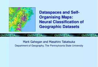
Dataspaces and Self- Organising Maps:Neural Classification of Geographic Datasets Mark Gahegan and Masahiro Takatsuka Department of Geography, The Pennsylvania State University
Wrestling with Feature Space • As a result of improved data capture, the feature space that analysis tools must address becomes deeper and more complex. • One traditional approach to manage this complexity is to break down feature space by theme… • … resulting in a number of distinct ‘data spaces’, such as spectral, hydrological, morphological, taxonomic and so forth. • Such themes traditionally possess strong internal structure.
Still wrestling with feature space... • By contrast, statistical classifiers and inductive learningtechniques usually treat the entire feature space as comprising a single descriptive vector <x, y, f1, f2, …, fn> • In geographic terms this is equivalent to the construction of an all-inclusive or universal dataspace. • In computational terms it makes finding a minimum cost solution more complex… each new feature adds a further dimension to the search problem. • Inductive classifiers operate by searching a hypothesis space of potential solutions.
Should feature space be structured? • Whilst strong clustering may exist within parts of the total space, it may be confounded by the 'noise' of unrelated (or weakly related) concepts. • This complicates the learning task, which in turn may reduce classification accuracy. • The counter argument to this is that each dimension may be useful for some discrimination task or other; some classification tasks may require most or all of the dimensions in the data concurrently. • hypothesis: Classification based on dataspaces can out-perform approaches using the entire feature space.
Divide and Conquer? • Different types of structuring can be applied in each feature sub-space: • E.g. a spectral dataspace may contain ratio data with an (approximately) Gaussian distribution, whereas a locational (geographic) space may show localized clustering and directional trends, requiring a different model. • Following a local process of classification or clustering within each space, a new space of part-classified dataspaces can be produced... • … and then mapped via a final classification stage to the target output classes.
Combined attribute vector as input to a self-organising map. Attribute vector split into three separate dataspaces, part-classified separately by three self-organising maps and then combined. Network architecture
Self-Organising Maps • As used here, the initial stage of the classifier attempts to 'mine' structure (by means of clustering) within each dataspace... • ...primarily, in isolation from final target classes. • The approach chosen is that of Self-Organising Maps (SOMs) (Kohonen, 1995) • Clustering and supervised learning are based around Vector Quantization-- mapping from a high dimensionality space to a 2D space.
Reference vectors Feature v2 Feature v1 Self-Organising Maps • Reference vectors partition the feature space into disjoint regions • One of the reference vectors within a region becomes the nearest-neighbour of any training samples falling in that region. • Reference vectors behave like generators in an ordinary Voronoi diagram except > 1 vectors can be used to describe a single class.
Supervised learning method • The task of learning is to position the reference vectors so that the tessellation they provide minimises the classification error. • An input vector x is classified by finding the reference vector wc that is the nearest-neighbour of x, as defined by the Euclidean metric: • The positioning of reference vectors is achieved using the optimised learning rate (OLVQ1) supervised learning algorithm.
Learning rules • The algorithm simulates learning as a dynamic process that takes place over a number of time slices (ti). • Initially, a number of reference vectors are introduced as {wi(t): i = 1,…, N}. The class of each reference vector is calculated using the k-nearest neighbour method (MacQueen, 1967), then their positions are updated according to the learning rules:
Experiments- The Dataset • The Kioloa Pathfinder Dataset is used for reporting purposes here, to facilitate direct comparison of classifier performance with previous work. • This dataset contains a number of thematic environmental surfaces that can be grouped into dataspaces and has a well-documented set of groundcover samples (1703) for training. • The combined attribute space is complex, and defies a simplistic approach to classification. (Classes overlap, are poorly delineated, and do not always form a single cluster.) • Training samples have a large input vector (11 surfaces) and contain the full range of statistical types. • The target domain is that of floristic classification, the differentiation of individual vegetation types (or vegetation niches), rather than the gross identification of urban, rural and water that are sometimes reported.
Initial Classification • Classification accuracy was first calculated on the entire feature space. • Two thirds of all examples were used in training, with one third held over for validation. • To examine the effects of different training – validation splits the data were randomly reorganised 10 times to produce 10 distinct classifiers. (Best result for both training and validation are shown in bold.) (AR= 77.51T, 64.25V) • Maximum Likelihood Classification gives about 40% accuracy.
Scaling of input data • SOM may develop poor mappings if elements of an input vector have different scales (Kohonen, 1995). • This situation often arises when an input vector consists of signals from different domains. • Standardising the dynamic range of each feature in the input vector ensures that any movements in a given direction in feature space are co-measurable. (AR: 82.42T, 67.82V)
Examining in more detail • Examining the individual class accuracy reveals some serious difficulties in classifying certain landcover types. • Classes with fewer training examples (particularly classes 2 and 3) attract fewer reference vectors, and hence may be described poorly. • Like most neural classifiers, SOMs have an inductive bias towards classes with larger samples; these offer the greatest potential for gains in accuracy.
Classification using data spaces • The next experiment uses a feature vector that is partitioned into several dataspaces. • each dataspace is first classified or clustered in isolation, then the output from the dataspaces becomes the input for a final combination phase. • an unsupervised SOM clusters regions of each dataspace, then Learning Vector Quantisation is used to combine the outputs generated (class labels are introduced). • Results were obtained for different distinct splits of the feature vector into dataspaces. • It is impractical to test all combinations; an attribute vector of size n and the condition that each layer be assigned to exactly one space would require n! separate experiments (9!= 362,880).
Dataspace example result • The results shown are for the following split: • dataspace 1 [North Aspect, East Aspect] • dataspace 2 [elevation, slope, surface water accumulation, geology, surface shape] • dataspace 3 [Landsat bands 2, 4, 5 and 7]}. • Performance on the training set improves (AR: 84.87T), giving a higher average score and with even less variance (< 2%). Validation shows that the classifier also outperforms the initial benchmark slightly (AR: 64.65) but does not achieve the same level of performance as the second experiment using scaled input vectors.
Observations • Some over-training may have occurred, indicated by higher training scores and lower validation scores. (Various different arrangements of neurons cause results to change.) • Performance is very stable for training. • Input vectors are not scaled, so a performance penalty should be expected. Interestingly, the dataspace splits that performed best had co-measurable dynamic ranges as well as strong geographic themes. • The unsupervised stage is operating blind-- it is not directed towards the target of floristic classification. However, the clusters formed must be useful, indicating that the dataspaces have internal structure that can be learned and applied.
SOM Advantages • Can operate effectively as a data reduction tool. • The classifiers appear to be stable. Without much effort in terms of experimental setup and network architecture we were able to achieve consistent results and reliable convergence • Convergence is rapid… around 10 seconds on a 400MHz PC for the dataset used here, (similar to decision trees and faster than standard backpropagation neural networks). • Can easily switch between supervised and unsupervised operation. • Can be built into a hierarchy for use with feature space decomposition… without paying a performance overhead.
SOM drawbacks • SOMs are particularly sensitive to differences in dynamic range of the input variables. • Better results follow when ranges are either co-measurable or standarised. • In terms of floristic classification the SOM performs poorly where classes are poorly separable. • Tools that can accommodate some uncertainty (such as DONNET, German et al., 1997) are able to achieve further improvements in validation accuracy. • The user must experiment: • learning rate must be set (can vary for each vector) • number of neurons used for LVQ must be set.
Future Work • The SOM architecture shows promise… allowing data to be structured without complicating the training phase or degrading performance. • Each dataspace can be treated differently, perhaps using alternative self-organising principles, perhaps favouring different styles of generalisation. • Statistics (e.g. co-variance) could be used to select candidate dataspaces.