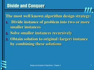
1. Divide and Conquer Andreas Klappenecker [based on slides by Prof. Welch]

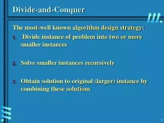
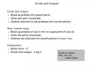
2. Divide and Conquer Paradigm • An important general technique for designing algorithms: • divide problem into subproblems • recursively solve subproblems • combine solutions to subproblems to get solution to original problem • Use recurrences to analyze the running time of such algorithms

3. Mergesort

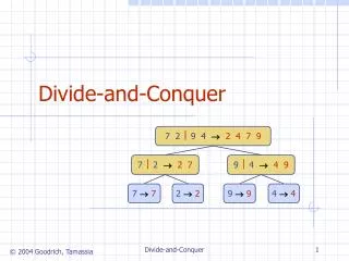
4. Example: Mergesort • DIVIDE the input sequence in half • RECURSIVELY sort the two halves • basis of the recursion is sequence with 1 key • COMBINE the two sorted subsequences by merging them

5. 1 5 2 2 4 2 3 6 4 1 5 3 6 2 6 6 2 5 2 4 4 5 6 6 1 1 2 3 3 2 6 6 5 2 5 2 5 2 4 4 6 6 1 1 3 3 2 2 6 6 4 6 2 6 1 3 Mergesort Example

6. Mergesort Animation • http://ccl.northwestern.edu/netlogo/models/run.cgi?MergeSort.862.378

7. Recurrence Relation for Mergesort • Let T(n) be worst case time on a sequence of n keys • If n = 1, then T(n) = (1) (constant) • If n > 1, then T(n) = 2 T(n/2) + (n) • two subproblems of size n/2 each that are solved recursively • (n) time to do the merge

8. Recurrence Relations

9. How To Solve Recurrences • Ad hoc method: • expand several times • guess the pattern • can verify with proof by induction • Master theorem • general formula that works if recurrence has the form T(n) = aT(n/b) + f(n) • a is number of subproblems • n/b is size of each subproblem • f(n) is cost of non-recursive part

10. Master Theorem Consider a recurrence of the form T(n) = a T(n/b) + f(n) with a>=1, b>1, and f(n) eventually positive. • If f(n) = O(nlogb(a)-), then T(n)=(nlogb(a)). • If f(n) = (nlogb(a) ), then T(n)=(nlogb(a) log(n)). • If f(n) = (nlogb(a)+) and f(n) is regular, then T(n)=(f(n)) [f(n) regular iff eventually af(n/b)<= cf(n) for some constant c<1]

11. Excuse me, what did it say??? Essentially, the Master theorem compares the function f(n) with the function g(n)=nlogb(a). Roughly, the theorem says: • If f(n) << g(n) then T(n)=(g(n)). • If f(n)  g(n) then T(n)=(g(n)log(n)). • If f(n) >> g(n) then T(n)=(f(n)). Now go back and memorize the theorem!

12. Déjà vu: Master Theorem Consider a recurrence of the form T(n) = a T(n/b) + f(n) with a>=1, b>1, and f(n) eventually positive. • If f(n) = O(nlogb(a)-), then T(n)=(nlogb(a)). • If f(n) = (nlogb(a) ), then T(n)=(nlogb(a) log(n)). • If f(n) = (nlogb(a)+) and f(n) is regular, then T(n)=(f(n)) [f(n) regular iff eventually af(n/b)<= cf(n) for some constant c<1]

13. Nothing is perfect… The Master theorem does not cover all possible cases. For example, if f(n) = (nlogb(a) log n), then we lie between cases 2) and 3), but the theorem does not apply. There exist better versions of the Master theorem that cover more cases, but these are even harder to memorize.

14. Idea of the Proof Let us iteratively substitute the recurrence:

15. Idea of the Proof Thus, we obtained T(n) = nlogb(a) T(1) + ai f(n/bi) The proof proceeds by distinguishing three cases: • The first term in dominant: f(n) = O(nlogb(a)-) • Each part of the summation is equally dominant: f(n) = (nlogb(a) ) • The summation can be bounded by a geometric series: f(n) = (nlogb(a)+) and the regularity of f is key to make the argument work.

16. Further Divide and Conquer Examples

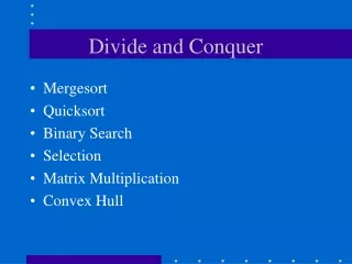
17. Additional D&C Algorithms • binary search • divide sequence into two halves by comparing search key to midpoint • recursively search in one of the two halves • combine step is empty • quicksort • divide sequence into two parts by comparing pivot to each key • recursively sort the two parts • combine step is empty

18. Additional D&C applications • computational geometry • finding closest pair of points • finding convex hull • mathematical calculations • converting binary to decimal • integer multiplication • matrix multiplication • matrix inversion • Fast Fourier Transform

19. Strassen’s Matrix Multiplication

20. Matrix Multiplication • Consider two n by n matrices A and B • Definition of AxB is n by n matrix C whose (i,j)-th entry is computed like this: • consider row i of A and column j of B • multiply together the first entries of the rown and column, the second entries, etc. • then add up all the products • Number of scalar operations (multiplies and adds) in straightforward algorithm is O(n3). • Can we do it faster?

21. Divide-and-Conquer • Divide matrices A and B into four submatrices each • We have 8 smaller matrix multiplications and 4 additions. Is it faster? A  B= C  =

22. Divide-and-Conquer Let us investigate this recursive version of the matrix multiplication. Since we divide A, B and C into 4 submatrices each, we can compute the resulting matrix C by • 8 matrix multiplications on the submatrices of A and B, • plus (n2) scalar operations

23. Divide-and-Conquer • Running time of recursive version of straightfoward algorithm is • T(n) = 8T(n/2) + (n2) • T(2) = (1) where T(n) is running time on an n x n matrix • Master theorem gives us: T(n) = (n3) • Can we do fewer recursive calls (fewer multiplications of the n/2 x n/2 submatrices)?

24. Strassen’s Matrix Multiplication A  B= C  = P1 = (A11+ A22)(B11+B22) P2 = (A21 + A22) * B11P3 = A11 * (B12 - B22) P4 = A22 * (B21 - B11) P5 = (A11 + A12) * B22P6 = (A21 - A11) * (B11 + B12) P7 = (A12 - A22) * (B21 + B22) C11 = P1 + P4 - P5 + P7C12 = P3 + P5C21 = P2 + P4C22 = P1 + P3 - P2 + P6

25. Strassen's Matrix Multiplication • Strassen found a way to get all the required information with only 7 matrix multiplications, instead of 8. • Recurrence for new algorithm is • T(n) = 7T(n/2) + (n2)

26. Solving the Recurrence Relation Applying the Master Theorem to T(n) = a T(n/b) + f(n) with a=7, b=2, and f(n)=(n2). Since f(n) = O(nlogb(a)-) = O(nlog2(7)-), case a) applies and we get T(n)= (nlogb(a)) = (nlog2(7)) = O(n2.81).

27. Discussion of Strassen's Algorithm • Not always practical • constant factor is larger than for naïve method • specially designed methods are better on sparse matrices • issues of numerical (in)stability • recursion uses lots of space • Not the fastest known method • Fastest known is O(n2.376) • Best known lower bound is (n2)