Divide-and-Conquer

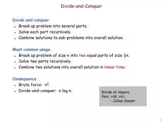
1. Divide-and-Conquer • Divide-and-conquer. • Break up problem into several parts. • Solve each part recursively. • Combine solutions to sub-problems into overall solution. • Most common usage. • Break up problem of size n into two equal parts of size ½n. • Solve two parts recursively. • Combine two solutions into overall solution in linear time. • Consequence. • Brute force: n2. • Divide-and-conquer: n log n. Divide et impera. Veni, vidi, vici. - Julius Caesar

2. Sorting • Sorting. Given n elements, rearrange in ascending order. • Obvious sorting applications. • List files in a directory. • Organize an MP3 library. • List names in a phone book. • Display Google PageRank results. • Problems become easier once sorted. • Find the median. • Find the closest pair. • Binary search in a database. • Identify statistical outliers. • Find duplicates in a mailing list. • Non-obvious sorting applications. • Data compression. • Computer graphics. • Interval scheduling. • Computational biology. • Minimum spanning tree. • Supply chain management. • Simulate a system of particles. • Book recommendations on Amazon. • Load balancing on a parallel computer.. . .

3. 5.3 Counting Inversions

4. Counting Inversions • Music site tries to match your song preferences with others. • You rank n songs. • Music site consults database to find people with similar tastes. • Similarity metric: number of inversions between two rankings. • My rank: 1, 2, …, n. • Your rank: a1, a2, …, an. • Songs i and j inverted if i < j, but ai > aj. • Brute force: check all (n2) pairs i and j. Songs A B C D E Inversions 3-2, 4-2 Me 1 2 3 4 5 You 1 3 4 2 5

5. Applications • Applications. • Voting theory. • Collaborative filtering. • Measuring the "sortedness" of an array. • Sensitivity analysis of Google's ranking function. • Rank aggregation for meta-searching on the Web. • Nonparametric statistics (e.g., Kendall's Tau distance).

6. Counting Inversions: Divide-and-Conquer • Divide-and-conquer. 1 5 4 8 10 2 6 9 12 11 3 7

7. Counting Inversions: Divide-and-Conquer • Divide-and-conquer. • Divide: separate list into two pieces. Divide: O(1). 1 5 4 8 10 2 6 9 12 11 3 7 1 5 4 8 10 2 6 9 12 11 3 7

8. Counting Inversions: Divide-and-Conquer • Divide-and-conquer. • Divide: separate list into two pieces. • Conquer: recursively count inversions in each half. Divide: O(1). 1 5 4 8 10 2 6 9 12 11 3 7 1 5 4 8 10 2 6 9 12 11 3 7 Conquer: 2T(n / 2) 5 blue-blue inversions 8 green-green inversions 5-4, 5-2, 4-2, 8-2, 10-2 6-3, 9-3, 9-7, 12-3, 12-7, 12-11, 11-3, 11-7

9. Counting Inversions: Divide-and-Conquer • Divide-and-conquer. • Divide: separate list into two pieces. • Conquer: recursively count inversions in each half. • Combine: count inversions where ai and aj are in different halves, and return sum of three quantities. Divide: O(1). 1 5 4 8 10 2 6 9 12 11 3 7 1 5 4 8 10 2 6 9 12 11 3 7 Conquer: 2T(n / 2) 5 blue-blue inversions 8 green-green inversions 9 blue-green inversions 5-3, 4-3, 8-6, 8-3, 8-7, 10-6, 10-9, 10-3, 10-7 Combine: ??? Total = 5 + 8 + 9 = 22.

10. Counting Inversions: Combine Combine: count blue-green inversions • Assume each half is sorted. • Count inversions where ai and aj are in different halves. • Merge two sorted halves into sorted whole. to maintain sorted invariant 3 7 10 14 18 19 2 11 16 17 23 25 6 3 2 2 0 0 13 blue-green inversions: 6 + 3 + 2 + 2 + 0 + 0 Count: O(n) 2 3 7 10 11 14 16 17 18 19 23 25 Merge: O(n)

11. Counting Inversions: Implementation • Pre-condition. [Merge-and-Count]A and B are sorted. • Post-condition. [Sort-and-Count]L is sorted. Sort-and-Count(L) { if list L has one element return 0 and the list L Divide the list into two halves A and B (rA, A)  Sort-and-Count(A) (rB, B)  Sort-and-Count(B) (rB, L)  Merge-and-Count(A, B) return r = rA + rB + r and the sorted list L }

12. 5.4 Closest Pair of Points

13. Closest Pair of Points • Closest pair. Given n points in the plane, find a pair with smallest Euclidean distance between them. • Fundamental geometric primitive. • Graphics, computer vision, geographic information systems, molecular modeling, air traffic control. • Special case of nearest neighbor, Euclidean MST, Voronoi. • Brute force. Check all pairs of points p and q with (n2) comparisons. • 1-D version. O(n log n) easy if points are on a line. • Assumption. No two points have same x coordinate. fast closest pair inspired fast algorithms for these problems to make presentation cleaner

14. Closest Pair of Points: First Attempt • Divide. Sub-divide region into 4 quadrants. L

15. Closest Pair of Points: First Attempt • Divide. Sub-divide region into 4 quadrants. • Obstacle. Impossible to ensure n/4 points in each piece. L

16. Closest Pair of Points • Algorithm. • Divide: draw vertical line L so that roughly ½n points on each side. L

17. 21 12 Closest Pair of Points • Algorithm. • Divide: draw vertical line L so that roughly ½n points on each side. • Conquer: find closest pair in each side recursively. L

18. 8 21 12 Closest Pair of Points • Algorithm. • Divide: draw vertical line L so that roughly ½n points on each side. • Conquer: find closest pair in each side recursively. • Combine: find closest pair with one point in each side. • Return best of 3 solutions. seems like (n2) L

19. 21 12 Closest Pair of Points • Find closest pair with one point in each side, assuming that distance < . L  = min(12, 21)

20. 21 12 Closest Pair of Points • Find closest pair with one point in each side, assuming that distance < . • Observation: only need to consider points within  of line L. L  = min(12, 21) 

21. 21 12 Closest Pair of Points • Find closest pair with one point in each side, assuming that distance < . • Observation: only need to consider points within  of line L. • Sort points in 2-strip by their y coordinate. L 7 6 5 4  = min(12, 21) 3 2 1 

22. 21 12 Closest Pair of Points • Find closest pair with one point in each side, assuming that distance < . • Observation: only need to consider points within  of line L. • Sort points in 2-strip by their y coordinate. • Only check distances of those within 11 positions in sorted list! L 7 6 5 4  = min(12, 21) 3 2 1 

23. Closest Pair of Points • Def. Let si be the point in the 2-strip, withthe ith smallest y-coordinate. • Claim. If |i – j|  12, then the distance betweensi and sj is at least . • Pf. • No two points lie in same ½-by-½ box. • Two points at least 2 rows aparthave distance  2(½). ▪ • Fact. Still true if we replace 12 with 7. j 39 31 ½ 2 rows 30 ½ 29 ½ i 28 27 26 25  

24. Closest Pair Algorithm Closest-Pair(p1, …, pn) { Compute separation line L such that half the points are on one side and half on the other side. 1 = Closest-Pair(left half) 2 = Closest-Pair(right half) = min(1, 2) Delete all points further than  from separation line L Sort remaining points by y-coordinate. Scan points in y-order and compare distance between each point and next 11 neighbors. If any of these distances is less than , update . return. } O(n log n) 2T(n / 2) O(n) O(n log n) O(n)

25. Closest Pair of Points: Analysis • Running time. • Q. Can we achieve O(n log n)? • A. Yes. Don't sort points in strip from scratch each time. • Each recursive returns two lists: all points sorted by y coordinate, and all points sorted by x coordinate. • Sort by merging two pre-sorted lists.

26. Matrix Multiplication

27. Matrix Multiplication • Matrix multiplication. Given two n-by-n matrices A and B, compute C = AB. • Brute force. (n3) arithmetic operations. • Fundamental question. Can we improve upon brute force?

28. Matrix Multiplication: Warmup • Divide-and-conquer. • Divide: partition A and B into ½n-by-½n blocks. • Conquer: multiply 8 ½n-by-½n recursively. • Combine: add appropriate products using 4 matrix additions.

29. Matrix Multiplication: Key Idea • Key idea. multiply 2-by-2 block matrices with only 7 multiplications. • 7 multiplications. • 18 = 10 + 8 additions (or subtractions).

30. Fast Matrix Multiplication • Fast matrix multiplication. (Strassen, 1969) • Divide: partition A and B into ½n-by-½n blocks. • Compute: 14 ½n-by-½n matrices via 10 matrix additions. • Conquer: multiply 7 ½n-by-½n matrices recursively. • Combine: 7 products into 4 terms using 8 matrix additions. • Analysis. • Assume n is a power of 2. • T(n) = # arithmetic operations.

31. Fast Matrix Multiplication in Practice • Implementation issues. • Sparsity. • Caching effects. • Numerical stability. • Odd matrix dimensions. • Crossover to classical algorithm around n = 128. • Common misperception: "Strassen is only a theoretical curiosity." • Advanced Computation Group at Apple Computer reports 8x speedup on G4 Velocity Engine when n ~ 2,500. • Range of instances where it's useful is a subject of controversy. • Remark. Can "Strassenize" Ax=b, determinant, eigenvalues, and other matrix ops.

32. Fast Matrix Multiplication in Theory • Q. Multiply two 2-by-2 matrices with only 7 scalar multiplications? • A. Yes! [Strassen, 1969] • Q. Multiply two 2-by-2 matrices with only 6 scalar multiplications? • A. Impossible. [Hopcroft and Kerr, 1971] • Q. Two 3-by-3 matrices with only 21 scalar multiplications? • A. Also impossible. • Q. Two 70-by-70 matrices with only 143,640 scalar multiplications? • A. Yes! [Pan, 1980] • Decimal wars. • December, 1979: O(n2.521813). • January, 1980: O(n2.521801).

33. Fast Matrix Multiplication in Theory • Best known. O(n2.376) [Coppersmith-Winograd, 1987.] • Conjecture. O(n2+) for any  > 0. • Caveat. Theoretical improvements to Strassen are progressively less practical.