Download
1 / 22
220 likes | 353 Vues
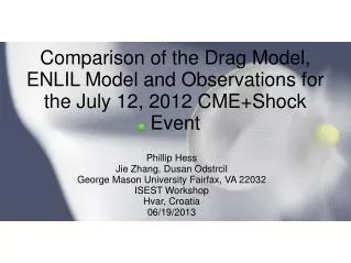
Phillip Hess Jie Zhang, Dusan Odstrcil George Mason University Fairfax, VA 22032 ISEST Workshop Hvar, Croatia 06/19/2013. Comparison of the Drag Model, ENLIL Model and Observations for the July 12, 2012 CME+Shock Event. Purpose.

E N D
Phillip Hess Jie Zhang, Dusan Odstrcil George Mason University Fairfax, VA 22032 ISEST Workshop Hvar, Croatia 06/19/2013 Comparison of the Drag Model, ENLIL Model and Observations for the July 12, 2012 CME+Shock Event
Purpose • To use prior events for which we have multiple data sets to constrain the physics of the Aerodynamic Drag Model to make CME and shock arrival predictions based only on initial conditions as accurate as possible • Provide a comparison between observations, analytic and numeric models for a well observed CME event
Snapshot of CME at 17:54 UT from three viewpoints fit with GCS Model (Thernisien 2006, 2009)
Aerodynamic Drag Model Where γ is the drag parameter, v0 is the initial CME speed, vsw is the ambient solar wind speed, r0 is the initial CME speed (Vrsnak et al 2012) Where cd is the drag coefficient, A is the CME cross-section, ρsw is the ambient solar wind density, ρ is the initial CME density, L is the CME thickness, ρsw0 is the initial ambient solar wind density, and ρ0 is the initial CME density, ρsw1AU is the ambient solar wind at 1AU, and ρ1AU is the CME density at 1 AU. The first three steps are described in detail in Vrsnak et al, the fourth and fifth were obtained by making three assumptions: (1) That L (CME thickness) could be approximated by r. This is essentially a spherical assumption. (2) That ρsw ~ 1/r2 and (3) That ρ0 ~ 1/r3 Or, to make fitting simpler γ can be treated as a constant
Comparison of Parameters For both fronts, ENLIL over estimates the velocity by 10-15% but the drag model does well, whether the data points are being fit to data with a constant γ or γ varies to provide the best comparison with in-situ arrival For both fronts, the constant γ falls between the min and max γ but the average value of the varying γ is above the constant γ
Conclusions • If more events are studied, a unique CD can be determined for each event based on initial knowledge, improving the accuracy of predictions • For this predictive scheme to work, the best way of determining the initial CME velocity and density and the ambient solar wind density and velocity will have to be determined • By comparing, observations to analytical and numerical models, we can understand more about all three