Download

1 / 29
300 likes | 557 Vues
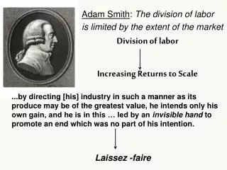
Increasing Returns and Home Markets. Edward Chamberlin. Doris Lessing (left) and Paul Krugman (right). Challenges to neoclassical trade theory:.

E N D
Increasing Returnsand Home Markets Edward Chamberlin Doris Lessing (left) and Paul Krugman (right)
Challenges to neoclassical trade theory: • Neoclasical trade theory (NTT) stresses country asymmetries, while the bulk of trade flows between similar countries, and it involves little net factor trade (70% of trade is intraindustry trade; see Grubel and Lloyd, 1974); • NTT misses important aspects of the effects of trade liberalization (within industry reallocations; Balassa, 1964); • NTT does not motivate the gravity model • It is also hard to think about firms (intrafirmtrade, multinational activity). • We will discuss models with scale economies, imperfect competition and product differentiation, which have proved to be very useful for dealing with these caveats. • These models do not attempt to replace neoclassical trade theory - effort to embed new features in the factor proportions framework (see Helpmanand Krugman, 1985). • A natural first step: study external (or Marshallian) economies of scale, which are consistent with perfect competition and homogenous products.
External Economies of Scale • The unit cost function is Where is a vector of external effects that affect the productivity of firms in sector I and country k. • Assume that and which means that the domestic externalities are positive. • Firms do not internalize the output spillovers on productivity, and so behave as if costs feature constant returns to scale.
External Economies of Scale: Autarchy • Assume two goods labeled 1 and 2, two countries (H,F), and one factor of production (Labor). • Assume that the cost functions take the following form for the goods: • Assume preferences are Cobb-Douglas with share for product 1. • Autarchy equilibrium conditions • Substituting for product 2,
External Economies of Scale: Trade • Open each country up for trade and Home specializes in good 1: • Solving for and plugging it into the price equation, we get: • Because we want Home to specialize in product 1,
External Economies of Scale: Welfare Analysis We know that the bold is larger than 1, indicating that Home is better off relative to autarchy. Foreign may be worse off if Home is an inefficient place for the IRS sector:
Monopolistic Competition: Introduction • Balassa (1964) proposed monopolistic competition as a setup for explaining the observed trade flows within the European common market. • These types of models gained prominence in the 1980s, because they can explain trade between similar countries and intraindustry trade: • even within industries, firms may produce varieties of the industry’s product; • if consumers value “variety” or tastes over varieties are heterogeneous, many brands are consumed; • with increasing returns, production of an individual variety is concentrated in one location and therefore brands are internationally traded. • These features lead naturally to intra-industry trade, and can generate large volumes of trade between similar countries.
Monopolistic Competition • With internal economies of scale there cannot be perfect competition. • Chamberlain (1933) proposed monopolistic competition as the market structure: • Every firm has some market power; it faces a downward sloping demand curve. • There is a large number of firms so that a price change by a single firm has no effect on the level of demand faced by the other firms. • There is free entry so that firms’ profits are driven down to zero (the large group case). • With product differentiation a firm has an incentive to differentiate its brand.
Monopolistic Competition Model Krugman 1979 Suppose there are i = 1,…,N product varieties, where N is endogenous. There are L consumers, each of whom has identical utility from consumption: Each consumer recieves labor income w, so the consumer can only consume Consumers maximize Utility, generating FOC: Totally differentiate and we get that the effect of a change in price is Define as the elasticity of demand. Notice that Elasticity depends on Consumption! Firms require labor to produce:
Monopolistic Competition Firm Behavior • Given wages w, average costs are • Each firm maximizes profits, setting marginal revenue equal to marginal cost. • In the long run, free entry drives profits to 0, so price equals average cost. Full employment, denoting demand for each good by Lc:
Effects of Opening Trade • Opening Trade is like increasing L and expanding access to varieties of goods. • Equilibrium consumption of every variety falls as expenditures are spread across product varieties. • This lowers prices, raising the real wage. • While trade allows access to more goods than before, the total number of varieties produced declines. As firms exploit the economies of scale, we would expect there to be fewer (selection), more productive (scale) firms.
Selection or Scale? • Evidence from Canada-U.S. FTA shows that the scale effect for Canadian firms was washed out by a decline in firm size as a response to lowering Canadian tariffs. • The actual scale effects seem not to be normatively important. • In Krugman, the selection effect does not enhance productivity, because firms are identical. This is a subject we will return to later in the course.
Product Differentiation: Love of Variety • Suppose the elasticity of substitution across varieties is constant . This means that scale effects are no longer relevant. • As , and varieties become perfect substitutes. • As , and utility is Cobb-Douglas • Suppose all products were equally desired: for all , we see a love of variety:
Product Differentiation • Where does the downward sloping demand come from? • Several approaches to product differentiation have been proposed. The most popular is the “love-of-variety” approach of Dixit and Stiglitz (1977) (see also Spence, 1976; and Lancaster, 1979). • Let there be I sectors of goods and denote by the set of varieties of good i, denote by a particular variety. • Preferences of a representative consumer are With We further assume CES preferences with a continuum of varieties.
Krugman (1980) • Consumers have CES preferences over varieties of a good Note that here consumption is denoted x, rather than c. • Technology: • Constant marginal cost of production in labor • Fixed cost of production f , paid in labor. • Monopolistic competition with a continuum of firms of measure n. Procedure: Solve utility maximization for each variety, proceed to maximize total production.
Closed Economy Solving demand for each variety: where P is the ideal price index, Increasing Returns Technology (Fixed Cost) with new notation:
Closed Economy Each firm maximizes profits subject to the above. Each firm is too small to affect wL or P, and so prices with a constant markup over marginal cost: Free entry means profits are 0: Labor market clearing: Welfare
Open Economy • H and F have different populations, • Free entry means that • Goods market clearing requires that all varieties have the same demand and factor price equalization holds: • Labor market Clearing means that in each country: • Home consumption is a fraction of world production of all varieties, generating two-way intraindustry trade. • Welfare • The effects are equivalent to doubling the population. • Note that welfare gains come from cheaper foreign products, not a change in the number of products available.
Gravity • Bilateral trade is directly proportional to the product of countries’ GDPs. • Assume a multicountry framework, with countries and products. denotes country I’s production of good k, with prices normalized to one. GDP is is share of country j’s share of world expenditure. Exports from country i to country j of product k are: Summing over all products k
Operationalizing the Gravity Equation • If countries specialize, tastes are identical and homothetic, and there is free trade worldwide, then the volume of trade among countries in region A is Bilaterally, we can write the equation in logs:
Helpman-Krugman Home Market effect • Increasing returns to scale industries tend to locate in larger markets and export their goods to other countries. • With two countries trading, the larger market will produce a greater number of products and be a net exporter of the differentiated good. • Cobb-Douglas preferences over 2 sectors. • differentiated CES good sector share • Homogenous good sector CRS, freely tradable.
Costly trade • Iceberg transportation costs • The idea is that a tariff melts some of the value of the good, for every unit shipped, only units arrive. • Drive a wedge between markets. • Domestic price = p = • Export price =
Equilibrium Equations • Free entry pins down the amount of production: Normalize wages and prices to 1. Demand for domestic residence of domestic products is: Goods market clearing:
Home market effects • Let be the share of the home country in the increasing returns industry. • Let be the share of the home country in labor. • Solving the equilibrium goods market clearing gives us several solutions for and and a general relationship between and :
Intuition for Home Market Result • Intuition: from a symmetric equilibrium, increase size of home, • more demand/profits for home firms. • to restore free entry, entry of domestic firms. • When τ < +∞, markets are shared by domestic and foreign firms. • Firm entry has a lower impact on profits than consumer entry. • Firm entry must respond more than proportionally to size.
Higher tariffs create stronger home market effects. • τ high: most competitors to domestic firms are also domestic. • domestic firms lose a lot from entry of domestic firms. • to restore zero profits, entry must move a little. • τ low: many competitors to domestic firms are foreign. • domestic firms lose little from entry of domestic firms. • to restore zero profits, entry must move a lot.
Testing the Home Market effect • Higher home demand should cause a country to be a net exporter of a good. • Davis and Weinstein (1996) find that more demand leads to a greater than proportional increase in production. • However, in American and Canadian data, industries with higher demand exhibit more imports than exports Head and Ries (2002).


![[READ DOWNLOAD] Increasing Returns and Path Dependence in the Economy (Economic](https://cdn7.slideserve.com/12623459/read-download-increasing-returns-and-path-dt.jpg)