Data Quality for Collisional-Radiative Modeling: Addressing Atomic State Populations and Line Spectra Accuracy
This presentation focuses on the importance of data quality for collisional-radiative modeling, specifically concerning atomic state populations and line spectra accuracy. Topics include the relevance of rate equations, autoionizing states, continuum ionization, charge exchange, recombination processes, and more. The talk delves into the challenges and requirements of accurate energy calculations, radiative autoionization, collisional limits, and neutral beam injection scenarios. It discusses dielectronic recombination, comparisons between models, validation strategies, and the impact of different collisional and radiative processes on the overall model accuracy.

Data Quality for Collisional-Radiative Modeling: Addressing Atomic State Populations and Line Spectra Accuracy
E N D
Presentation Transcript
Data Quality and Needs for Collisional-Radiative Modeling Yuri Ralchenko National Institute of Standards and Technology Gaithersburg, MD, USA Joint ITAMP-IAEA Workshop, Cambridge MA July 9, 2014
Basic rate equation Vector of atomic states populations Rate matrix
autoionizing states Collisional- Radiative Model Continuum ionization limit dielectronic capture autoionization (de)excitation charge exchange rad. transitions recombination ionization Z Z+1
Collisional-radiative models are generally problem-taylored
Atomic states Term Superconfiguration 1P 1224344452 3s23p3d24p 3P 3D3 1D 12283541 3D2 3D 3D1 3S 122836 3s23p34s Average atom Level Configuration 5S BUT: field modifications, ionization potential lowering
How good are the energies? • The current accuracy of energies (better than 0.1%) is sufficient for population kinetics calculations • For detailed spectral analysis, having as accurate as possible wavelengths/energies is crucial(blends) • May need >1,000,000 states
Radiative Autoionization • Allowed: generally very good if the most advanced methods (MCHF, MCDHF, etc) are used • Forbidden: generally good, less important for kinetics • Acceptable for kinetics, (almost) no data for highly-charged ions
Collisions and density limits • High density • Different for different ion charges • LTE/Saha equilibrium • Collisions are much stronger than non-collisional processes • Populations only depend on energies, degeneracies, and (electron) temperature • BUT: need radiative rates for spectral emission • Low density (corona) • All data are (generally) important • Line intensities (mostly) do NOT depend on radiative rates, only on collisional rates pLTE Corona
e-He excitation and ionization • Completeness • Consistency • Quality • Evaluation
Neutral beam injection:Motional Stark Effect W. Mandl et al. PPCF 35 1373(1993) σ Iij,a.u. H π λ(Hα) Displacement of Hα Example: ; /0 = 0.353 0.42
Solution: eigenstates are the parabolic states E = v×B parabolicstatesnikimi = /2 for MSE Radiativechannelnikimi→ njkjmjπ – componentswithΔm=0σ – componentswithΔm=±1 nilimi– sphericalstates Standard approach: nilimi→ njljmj Only one axis: along projectile velocity There is another axis: along the induced electric field E How to calculate the collisional parameters for parabolic states?
Answer • Express scattering parameters (excitation cross sections) for parabolic states (nkm) quantized along z in terms of scattering parameters (excitation cross sections AND scattering amplitudes) for spherical states (nlm) quantized along z’ O. Marchuk et al, J.Phys. B 43, 011002 (2010)
Collisional-radiative model • Fast (~50-500 keV) neutral beam penetrates hot (2-20 keV) plasma • States: 210 parabolic nkm(recalculate energies for each beam energy/magnetic field combination) up to n=10 • Radiative rates + field-ionization rates are well known • Proton-impact collisions are most important • AOCC for 1-2 and 1-3 (D.R. Schultz) • Glauber (eikonal approximation) for others • Recombination is not important (ionization phase) • Quasy-steady state
Theory vs. JET and Alcator C-Mod E. Delabie et al (2010) I. Bespamyatnov et al(2013)
How to compare CR models?.. • Attend the Non-LTE Code Comparison Workshops! • Compare integral characteristics • Ionization distributions • Radiative power losses • Compare effective (averaged) rates • Compare deviations from equilibrium (LTE) • 8 NLTE Workshops • Chung et al, HEDP 9, 645 (2013) • Fontes et al, HEDP 5, 15 (2009) • Rubiano et al, HEDP 3, 225 (2007) • Bowen et al, JQSRT 99, 102 (2006) • Bowen et al, JQSRT 81, 71 (2003) • Lee et al, JQSRT 58, 737 (1997) • Typically ~25 participants, ~20 codes Validation and Verification
EBIT: DR resonances with M-shell (n=3) ions EBIT electron beam 1s22s22p63s23p63dn extracted ions LMN resonances: L electron into M, free electron into N Fast beam ramping ER ER ER time
Strategy Ca-like W54+ • Scan electron beam energy with a small step (a few eV) • When a beam hits a DR, ionization balance changes • Both the populations of all levels within an ion and the corresponding line intensities also change • Measure line intensity ratios from neighbor ions and look for resonances • EUV lines: forbidden magnetic-dipole lines within the ground configuration Ionization potential A(E1) ~ 1015s-1 A(M1) ~ 105-106 s-1 I = NAE (intensity)
[Ca]/[K] THEORY: no DR
[Ca]/[K] THEORY: no DR isotropic DR Non-Maxwellian (40-eV Gaussian) collisional-radiative model: ~10,500 levels
[Ca]/[K] Non-Maxwellian (40-eV Gaussian) collisional-radiative model: ~18,000 levels THEORY: no DR isotropic DR anisotropic DR J m=+J m=-J atomic level degenerate magnetic sublevels Impact beam electrons are monodirectional
Monte Carlo analysis: uncertainty propagation in CR models • Generate a (pseudo-)random number between 0 and 1 • Using Marsaglia polar method, generate a normal distribution • Randomly multiply every rate by the generated number(s) • To preserve physics, direct and reverse rates (e.g. electron-impact ionization and three-body recombination) are multiplied by the same number • Ionization distribution is calculated for steady-state approximation
We think in logarithms… • Sample probability distribution • Normal distribution with the standard deviation • Normal distribution is applied to log(Rate) • log-normal distribution
Ne: fixed Ion/Rec rates Ne = 108 cm-3 Te = 1-100 eV Ionization stages: Ne I-IX ONLY ground states MC: 106 runs NOMAD code (Ralchenko & Maron, 2001)
Only stdev=10 Structures appear!
Lines: two ions populated 1- Z Z+n n=1, 2, >2
Needs and conclusions (collisions) • CROSS SECTIONS, neither rates nor effective collision strengths • EBITs, neutral beams, kappa distributions,… • Scattering amplitudes (off-diagonal density matrix elements) • Also magnetic sublevels • Complete consistent (+evaluated) sets (e.g., all excitations up to a specific nmax) • Do we want to have an online “dump” depository? AMDU IAEA? VAMDC? • Need better communication channels