Molecular Evolution and Genomics: A Comprehensive 10-Day Curriculum
This detailed 10-day curriculum covers the fundamental concepts of molecular evolution, phylogenetics, and comparative genomics. Each day consists of lectures, practical sessions, and project preparations, guiding participants through statistical alignment techniques, gene genealogies, and systems biology concepts. Learners will engage in exercises, study significant literature, and collaborate on projects that explore themes such as the Jukes-Cantor model, inferring recombination histories, and integrative data analysis. This program provides a robust foundation for understanding evolutionary processes through data analysis in biology.

Molecular Evolution and Genomics: A Comprehensive 10-Day Curriculum
E N D
Presentation Transcript
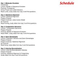
Schedule Day 1: Molecular Evolution Introduction Lecture: Models of Sequence Evolution Practical: Phylogenies Chose Project and collect literature Read Lunter, study slides from day 2 and find questions. Day 2: Statistical Alignment Lecture: Statistical Alignment Prepare Projects Prepare Exercise: Jukes-Cantor Model Do Exercise Read Ponting, study slides from day 3 and find questions. Day 3: Comparative Genomics Lecture: Comparative Genomics Prepare Projects Practical: Models of Sequence Evolution Read HSW1, study slides from day 3 and find questions. Day 4: Gene Genealogies Lecture: Population Genetics and Gene Genealogies Prepare Projects Prepare Exercise: Statistical Alignment Do Exercise Read Song, study slides from day 3 and find questions. Day 5: Inferring Recombination Lecture: Inferring Recombination Histories Prepare Projects Practical: Statistical Alignment & Footprinting Study slides from day 6 and find questions.
Schedule Day 6: Networks Lecture: Networks and other concepts Prepare Projects Prepare Exercise Do Exercise Study slides from day 7 and find questions. Day 7: Grammars and Hidden Structures in Biology Lecture (L): Prepare Projects Practical: Detecting Recombinations Study slides from day 8 and find questions. Day 8: Data analysis and Functional Explanation Lecture: Grammars and RNA Prediction Prepare Projects Prepare Exercise Do Exercise Study slides from day 9 and find questions. Day 9: Comparative Biology Lecture: Concepts, Data Analysis and Functional Studies Prepare Projects Practical – Integrative Data Analysis – Mapping Study project presentations of each other and find questions. Day 10: Systems Biology Project 1 – Population Genomics: Selective Sweeps Project 2 – Molecular Evolution: LUCA Project 3 – Integrative Genomics I: Basic data types Project 4 – Comparative Genomics: Dark Matter Project 5 - Integrative Genomics: Proteomics/Metabonomics
The Data & its growth. 1976/79 The first viral genome –MS2/fX174 1995 The first prokaryotic genome – H. influenzae 1996 The first unicellular eukaryotic genome - Yeast 1997 The first multicellular eukaryotic genome – C.elegans 2000 Arabidopsis thaliana, Drosophila 2001 The human genome 2002 Mouse Genome 2005+ Dog, Marsupial, Rat, Chicken, 12 Drosophilas 1.5.08: Known >10000 viral genomes 2000 prokaryotic genomes 80 Archeobacterial genomes A general increase in data involving higher structures and dynamics of biological systems
The Human Genome (Harding & Sanger) 3*109 bp Myoglobin a globin *50.000 b-globin (chromosome 11) 6*104 bp *20 Exon 3 Exon 1 Exon 2 3*103 bp 5’ flanking 3’ flanking *103 DNA: ATTGCCATGTCGATAATTGGACTATTTGGA 30 bp Protein: aa aa aa aa aa aa aa aa aa aa
ACGCC ACGCC AGGCC AGGCC AGGCT AGGCT AGGGC AGGCT AGGCT AGGTT AGGTT AGTGC Central Problems: History cannot be observed, only end products. ACGTC ACGTC Even if History could be observed, the underlying process couldn’t !!
Some Definitions State space – a set often corresponding of possible observations ie {A,C,G,T}. A random variable, X can take values in the state space with probabilities ie P{X=A} = ¼. The value taken often indicated by small letters - x Stochastic Process is a set of time labeled stochastic variables Xt ie P{X0=A, X1=C, .., X5=G} =.00122 Time can be discrete or continuous, in our context it will almost always mean natural numbers, N {0,1,2,3,4..}, or an interval on the real line, R. Markov Property: ie Time Homogeneity – the process is the same for all t.
Simplifying Assumptions I Probability of Data Biological setup TCGGTA TGGTT a - unknown 1) Only substitutions. s1 TCGGTA s1 TCGGA s2 TGGT-T s2 TGGTT a5 a4 a3 a2 a1 T A T G G G G C T T Data: s1=TCGGTA,s2=TGGTT 2) Processes in different positions of the molecule are independent, so the probability for the whole alignment will be the product of the probabilities of the individual patterns.
Simplifying Assumptions II a l2+l1 l1 = l2 s1i s2i s2i s1i 3) The evolutionary process is the same in all positions 4) Time reversibility: Virtually all models of sequence evolution are time reversible. I.e. πi Pi,j(t) = πj Pj,i(t), where πi is the stationary distribution of i and Pt(i->j) the probability that state i has changed into state j after t time. This implies that
Simplifying assumptions III t1 e A t2 C C 5) The nucleotide at any position evolves following a continuous time Markov Chain. Pi,j(t) continuous time markov chain on the state space {A,C,G,T}. Q - rate matrix: T O A C G T FA -(qA,C+qA,G+qA,T) qA,C qA,G qA,T RC qC,A -(qC,A+qC,G+qC,T) qC, G qC ,T OG qG,A qG,C -(qG,A+qG,C+qG,T) qG,T MT qT,A qT,C qT,G -(qT,A+qT,C+qT,G) 6) The rate matrix, Q, for the continuous time Markov Chain is the same at all times (and often all positions). However, it is possible to let the rate of events, ri, vary from site to site, then the term for passed time, t, will be substituted by ri*t.
Q and P(t) What is the probability of going from i (C?) to j (G?) in time t with rate matrix Q? i. P(0) = I ii. P(e) close to I+eQ for e small iii. P'(0) = Q. iv. lim P(t) has the equilibrium frequencies of the 4 nucleotides in each row v. Waiting time in state j, Tj, P(Tj > t) = eqjjt Expected number of events at equilibrium vi. QE=0Eij=1 (all i,j) vii. PE=E viii. If AB=BA, then eA+B=eAeB.
Jukes-Cantor (JC69): Total Symmetry Rate-matrix, R: T O A C G T F A -3*aa aa R C a -3*aaa O G a a -3* a a M T a a a -3* a Transition prob. after time t, a = a*t: P(equal) = ¼(1 + 3e-4*a ) ~ 1 - 3a P(specific difference) = ¼(1 - e-4*a ) ~ 3a Stationary Distribution: (1,1,1,1)/4.
Principle of Inference: Likelihood Likelihood function L() – the probability of data as function of parameters: L(Q,D) LogLikelihood Function – l(): ln(L(Q,D)) If the data is a series of independent experiments L() will become a product of Likelihoods of each experiment, l() will become the sum of LogLikelihoods of each experiment Likelihood LogLikelihood In Likelihood analysis parameter is not viewed as a random variable.
Exponentiation/Powering of Matrices By eigen values: where If then and Finding L: det (Q-lI)=0 Finding B: (Q-liI)bi=0 JC69: where k ~6-10 Numerically:
Kimura 2-parameter model - K80 TO A C G T F A -2*b-a b a b R Cb -2*b-a b a O Ga b -2*b-a b M Tb a b -2*b-a a = a*t b = b*t Q: start P(t)
Felsenstein81 & Hasegawa, Kishino & Yano 85 Unequal base composition: (Felsenstein, 1981 F81) Qi,j = C*πj i unequal j Rates to frequent nucleotides are high - (π=(πA , πC , πG , πT) T A Tv/Tr = (πT πC +πA πG )/[(πT+πC )(πA+ πG )] G C Tv/Tr & compostion bias (Hasegawa, Kishino & Yano, 1985 HKY85) (a/b)*C*πj i- >j a transition Qi,j = C*πj i- >j a transversion Tv/Tr = (a/b) (πT πC +πA πG )/[(πT+πC )(πA+πG )]
Measuring Selection ThrPro ACGCCA - ThrSer ACGCCG ArgSer AGGCCG - ThrSer ACTCTG AlaSer GCTCTG AlaSer GCACTG ThrSer ACGTCA Certain events have functional consequences and will be selected out. The strength and localization of this selection is of great interest. The selection criteria could in principle be anything, but the selection against amino acid changes is without comparison the most important
i. The Genetic Code 3 classes of sites: 4 2-2 1-1-1-1 4 (3rd) 1-1-1-1 (3rd) ii. TA (2nd) Problems: i. Not all fit into those categories. ii. Change in on site can change the status of another.
Possible events if the genetic code remade from Li,1997 Possible number of substitutions: 61 (codons)*3 (positions)*3 (alternative nucleotides). Substitutions Number Percent Total in all codons 549 100 Synonymous 134 25 Nonsynonymous 415 75 Missense 392 71 Nonsense 23 4
Probabilities: Rates: b start b a a b Kimura’s 2 parameter model & Li’s Model. Selection on the 3 kinds of sites (a,b)(?,?) 1-1-1-1 (f*a,f*b) 2-2 (a,f*b) 4 (a, b)
alpha-globin from rabbit and mouse. Ser Thr Glu Met Cys Leu Met Gly Gly TCA ACT GAG ATG TGT TTA ATG GGG GGA * * * * * * * ** TCG ACA GGG ATA TAT CTA ATG GGT ATA Ser Thr Gly Ile Tyr Leu Met Gly Ile Sites Total Conserved Transitions Transversions 1-1-1-1 274 246 (.8978) 12(.0438) 16(.0584) 2-2 77 51 (.6623) 21(.2727) 5(.0649) 4 78 47 (.6026) 16(.2051) 15(.1923) Z(at,bt) = .50[1+exp(-2at) - 2exp(-t(a+b)] transition Y(at,bt) = .25[1-exp(-2bt )] transversion X(at,bt) = .25[1+exp(-2at) + 2exp(-t(a+b)] identity L(observations,a,b,f)= C(429,274,77,78)* {X(a*f,b*f)246*Y(a*f,b*f)12*Z(a*f,b*f)16}* {X(a,b*f)51*Y(a,b*f)21*Z(a,b*f)5}*{X(a,b)47*Y(a,b)16*Z(a,b)15} where a = at and b = bt. Estimated Parameters: a = 0.3003 b = 0.1871 2*b = 0.3742 (a + 2*b) = 0.6745 f = 0.1663 Transitions Transversions 1-1-1-1 a*f = 0.0500 2*b*f = 0.0622 2-2 a = 0.3004 2*b*f = 0.0622 4 a = 0.3004 2*b = 0.3741 Expected number of: replacement substitutions 35.49 synonymous 75.93 Replacement sites : 246 + (0.3742/0.6744)*77 = 314.72 Silent sites : 429 - 314.72 = 114.28 Ks = .6644 Ka = .1127