Sequence Alignment Tutorial
Sequence Alignment Tutorial. Presented by Kirill Bessonov Oct 2012. Talk Structure. Introduction to sequence alignments Methods / Logistics Global Alignment: Needleman- Wunsch Local Alignment: Smith-Waterman Illustrations of two types of alignments s tep by step local alignment

Sequence Alignment Tutorial
E N D
Presentation Transcript
Sequence Alignment Tutorial Presented by Kirill Bessonov Oct 2012
Talk Structure • Introduction to sequence alignments • Methods / Logistics • Global Alignment: Needleman-Wunsch • Local Alignment: Smith-Waterman • Illustrations of two types of alignments • step by step local alignment • Computational implementation of alignment • Retrieval of sequences using R • Alignment of sequences using R • Homework
Sequence Alignments Comparing two objects is intuitive. Likewise sequence pairwise alignments provide info on: • evolutionary distance between species (e.g. homology) • new functional motifs / regions • genetic manipulation (e.g. alternative splicing) • new functional roles of unknown sequence • identification of binding sites of primers / TFs • de novo genome assembly • alignment of the short “reads” from high-throughput sequencer (e.g. Illumina or Roche platforms)
Comparing two sequences entire sequence perfect match unaligned rest of thesequence alignedportion • There are two ways of pairwise comparison • Global using Needleman-Wunschalgorithm (NW) • Local using Smith-Waterman algorithm (SW) • Both approaches use similar methodology, but have completely different objectives • Global alignment (NW) • tries to align the “whole” sequence • more restrictive than local alignment • Local alignment (SW) • tries to align portions (e.g. motifs) of given sequences • more flexible as considers “parts” of the sequence • works well on highly divergent sequences
Global alignment (NW) • Sequences are aligned end-to-end along their entire length • Many possible alignments are produced • The alignment with the highest score is chosen • Naïve algorithm is very inefficient (Oexp) • To align sequence of length 15, need to consider • Possibilities # = (insertion, deletion, gap)15 = 315 = 1,4*107 • Impractical for sequences of length >20 nt • Used to analyze homology/similarity of entire: • genes and proteins • assess gene/protein overall homology between species
Methodology of global alignment (1 of 4) • Define scoring scheme for each event • mismatch between ai and bj • if • gap (insertion or deletion) • match between ai and bj • if • Provide no restrictions on minimal score • Start completing the alignment MxN matrix
Methodology of global alignment (2 of 4) -2 -2 -2 -2 -2 -2 -2 • The matrix should have extra column and row • M+1 columns , where M is the length sequence M • N+1 rows, where N is the length of sequence N • Initialize the matrix by introducing gap penalty at every initial position along rows and columns • Scores at each cell are cumulative
Methodology of global alignment (3 of 4) +2 -2 -1 -2 • For each cell consider all three possibilities 1)Gap (horiz/vert) 2)Match (diag) 3)Mismatch(diag) • Select the maximum score for each cell and fill the matrix
Methodology of global alignment (4 of 4) • Select the most very bottom right cell • Consider different path(s) going to very top left cell • Path is constructed by finding the source cell w.r.t. the current cell • How the current cell value was generated? From where? WHAT WHAT WHY- WH-Y Overall score = 1 Overall score = 1 • Select the best alignment(s)
Local alignment (SW) • Sequences are aligned to find regions (part of the original sequence) where the best alignment occurs • Local similarity context (aligning parts) • More detailed / “micro” appoach • Ideal for finding short motifs, DNA binding sites • Works well on highly divergent sequences • Sequences with highly variable introns but highly conserved and sparse exons
Methodology of local alignment (1 of 4) • The scoring system is similar with one exception • The minimum possible score in the matrix is zero • There are no negative scores in the matrix • Let’s define the same scoring system as in global 1) mismatch between ai and bj2) gap (insertion or deletion) if 3) match between ai and bj if
Methodology of local alignment (2 of 4) Construct the MxN alignment matrix with M+1 columns and N+1 rows Initialize the matrix by introducing gap penalty at 1st row and 1st column
Methodology of local alignment (3 of 4) • For each subsequent cell consider all possibilities (i.e. motions) • Vertical 2)Horizontal 3)Diagonal • For each cell select the highest score • If score is negative assign zero
Methodology of local alignment (4 of 4) • I • A • J • total score of 4 • B • Select the initial cell with the highest score(s) • Consider different path(s) leading to score of zero • Trace-back the cell values • Look how the values were originated (i.e. path) WH WH • Mathematically • where S(I, J)is the score for subsequencesI and J
Local alignment illustration (1 of 2) • Determine the best local alignment and the maximum alignment score for • Sequence A: ACCTAAGG • Sequence B: GGCTCAATCA • Scoring conditions: • if , • if and
Local alignment illustration (3 of 3) in the whole seq. context CTCAA GGCTCAATCA CT-AA ACCT-AAGG Best score: 6
Protein Alignment • Protein local and global alignment follows the same rules as we saw with DNA/RNA • Differences • alphabet of proteins is 22 residues long • special scoring/substitution matrices used • conservation and protein proprieties are taken into account • E.g. residues that are totally different due to charge such as polar Lysine and apolar Glycine are given a low score
Substitution matrices • Since protein sequences are more complex, matrices are collection of scoring rules • These are 2D matrices reflecting comparison between sequence A and B • Cover events such as • mismatch and perfect match • Need to define gap penalty separately • Popular BLOcksSUbstitutionMatrix (BLOSUM)
BLOSUM-x matrices • Constructed from aligned sequences with specific x% similarity • matrix built using sequences with no more then 50% similarity is called BLOSUM-50 • For highly mutating / dissimilar sequences use • BLOSUM-45 and lower • For highly conserved / similar sequences use • BLOSUM -62 and higher
BLOSUM 62 perfect match between a.a. Score = 2 Score = -3 What diagonal represents? What is the score for substitution ED (acid a.a.)? More drastic substitution KI (basic to non-polar)?
Practical problem:Align following sequences both globally and locally using BLOSUM 62 matrix with gap penalty of -8Sequence A: AAEEKKLAAASequence B: AARRIA
Aligning globally using BLOSUM 62 AAEEKKLAAA AA--RRIA-- Score: -14 Other alignment options? Yes
Aligning locally using BLOSUM 62 KKLA RRIA Score: 10
Using R and SeqinRlibrary for: • Sequence Retrieval and Analysis
Protein database UniProt database (http://www.uniprot.org/) has high quality protein data manually curated It is manually curated Each protein is assigned UniProt ID
Retrieving data from Uniprot ID • In search field one can enter either use UniProt ID or common protein name • example: myelin basic protein • We will use retrieve data for P02686
Understanding fields Information is divided into categories Click on ‘Sequences’ category and then FASTA
FASTA format Actual protein sequence starts from 2nd line • FASTA format is widely used and has the following parameters • Sequence name start with > sign • The fist line corresponds to protein name
Retrieving protein data with R and SeqinR • Can “talk” to UniProt database using R • SeqinRlibrary is suitable for • “Biological Sequences Retrieval and Analysis” • Detailed manual could be found here • Install this library in your R environment install.packages("seqinr") library("seqinr") • Choose database to retrieve data from choosebank("swissprot") • Download data object for target protein (P02686) query("MBP_HUMAN", "AC=P02686") • See sequence of the object MBP_HUMAN MBP_HUMAN_seq = getSequence(MBP_HUMAN); MBP_HUMAN_seq
Dot Plot (comparison of 2 sequences) (1of2) • 2D way to find regions of similarity between two sequences • Each sequence plotted on either vertical or horizontal dimension • If two a.a. at given positions are identical the dot is plotted • matching sequence segments appear as diagonal lines
Dot Plot (comparison of 2 sequences) (2of2) • Visualize dot plot dotPlot(MBP_HUMAN_seq[[1]], MBP_MOUSE_seq[[1]],xlab="MBP - Human", ylab = "MBP - Mouse") • - Is there similarity between human and mouse form of MBP protein? - Where is the difference in the sequence between the two isoforms? • Let’s compare two protein sequences • Human MBP (Uniprot ID: P02686) • Mouse MBP (Uniprot ID: P04370) • Download 2nd mouse sequence query("MBP_MOUSE", "AC=P04370"); MBP_MOUSE_seq = getSequence(MBP_MOUSE);
Using R and Biostrings library for: • Pairwise global and local alignments
Installing Biostrings library DNA_subst_matrix • Install library from Bioconductor source("http://bioconductor.org/biocLite.R") biocLite("Biostrings") library(Biostrings) • Define substitution martix (e.g. for DNA) DNA_subst_matrix = nucleotideSubstitutionMatrix(match = 2, mismatch = -1, baseOnly = TRUE) • The scoring rules • Match: = 2 if • Mismatch: = -1 if • Gap: = -2 or = -2
Global alignment using R and Biostrings • Create two sting vectors (i.e. sequences) seqA = "GATTA" seqB = "GTTA" • Use pairwiseAlignment() and the defined rules globalAlignAB = pairwiseAlignment(seqA, seqB, substitutionMatrix= DNA_subst_matrix, gapOpening = -2, scoreOnly= FALSE, type="global") • Visualize best paths (i.e. alignments) globalAlignAB Global PairwiseAlignedFixedSubject (1 of 1) pattern: [1] GATTA subject: [1] G-TTA score: 2
Local alignment using R and Biostrings • Input two sequences seqA = "AGGATTTTAAAA" seqB = "TTTT" • The scoring rules will be the same as we used for global alignment globalAlignAB = pairwiseAlignment(seqA, seqB, substitutionMatrix = DNA_subst_matrix, gapOpening = -2, scoreOnly = FALSE, type="local") • Visualize alignment globalAlignAB Local PairwiseAlignedFixedSubject (1 of 1) pattern: [5] TTTT subject: [1] TTTT score: 8
Aligning protein sequences • Protein sequences alignments are very similar except the substitution matrix is specified data(BLOSUM62) BLOSUM62 • Will align sequences seqA = "PAWHEAE" seqB= "HEAGAWGHEE" • Execute the global alignment globalAlignAB <- pairwiseAlignment(seqA, seqB, substitutionMatrix= "BLOSUM62", gapOpening = -2, gapExtension= -8, scoreOnly = FALSE)
Summary • We had touched on practical aspects of • Global and local alignments • Thoroughly understood both algorithms • Applied them both on DNA and protein seq. • Learned on how to retrieve sequence data • Learned on how to retrieve sequences both with R and using UniProt • Learned how to align sequences using R
Resources • Online Tutorial on Sequence Alignment • http://a-little-book-of-r-for-bioinformatics.readthedocs.org/en/latest/src/chapter4.html • Graphical alignment of proteins • http://www.dina.kvl.dk/~sestoft/bsa/graphalign.html • Documentation on libraries • Biostings: http://www.bioconductor.org/packages/2.10/bioc/manuals/Biostrings/man/Biostrings.pdf • SeqinR:http://seqinr.r-forge.r-project.org/seqinr_2_0-7.pdf