Sequence Alignment: Needleman-Wunsch & Smith-Waterman + Dot Plot Analysis
Understand Needleman-Wunsch & Smith-Waterman algorithms, PAM & BLOSUM scoring matrices, affine gap penalties, and dot plot comparisons. Learn how to analyze sequences using dot plots with Dotlet tool. Explore protein sequence alignments and scoring methods.

Sequence Alignment: Needleman-Wunsch & Smith-Waterman + Dot Plot Analysis
E N D
Presentation Transcript
Example x = AGTA m = 1 y = ATA s = -1 d = -1 F(i,j) i = 0 1 2 3 4 F(1, 1) = max{F(0,0) + s(A, A), F(0, 1) – d, F(1, 0) – d} = max{0 + 1, -1 – 1, -1 – 1} = 1 j = 0 1 2 A A G - T T A A 3
The Needleman-Wunsch Matrix x1 ……………………………… xM Every nondecreasing path from (0,0) to (M, N) corresponds to an alignment of the two sequences y1 ……………………………… yN An optimal alignment is composed of optimal subalignments
AKRANR KAAANK -1 + (-1) + (-2) + 5 + 7 + 3 = 11 Scoring Matrix: Example • Notice that although R and K are different amino acids, they have a positive score. • Why? They are both positively charged amino acids will not greatly change function of protein.
PAM • Point Accepted Mutation (Dayhoff et al.) • 1 PAM = PAM1 = 1% average change of all amino acid positions • After 100 PAMs of evolution, not every residue will have changed • some residues may have mutated several times • some residues may have returned to their original state • some residues may not changed at all
PAMX • PAMx = PAM1x • PAM250 = PAM1250 • PAM250 is a widely used scoring matrix: Ala Arg Asn Asp Cys Gln Glu Gly His Ile Leu Lys ... A R N D C Q E G H I L K ... Ala A 13 6 9 9 5 8 9 12 6 8 6 7 ... Arg R 3 17 4 3 2 5 3 2 6 3 2 9 Asn N 4 4 6 7 2 5 6 4 6 3 2 5 Asp D 5 4 8 11 1 7 10 5 6 3 2 5 Cys C 2 1 1 1 52 1 1 2 2 2 1 1 Gln Q 3 5 5 6 1 10 7 3 7 2 3 5 ... Trp W 0 2 0 0 0 0 0 0 1 0 1 0 Tyr Y 1 1 2 1 3 1 1 1 3 2 2 1 Val V 7 4 4 4 4 4 4 4 5 4 15 10
BLOSUM • Blocks Substitution Matrix • Scores derived from observations of the frequencies of substitutions in blocks of local alignments in related proteins • Matrix name indicates evolutionary distance • BLOSUM62 was created using sequences sharing no more than 62% identity
Local Alignment: Free Rides Yeah, a free ride! Vertex (0,0) The dashed edges represent the free rides from (0,0) to every other node.
Notice there is only this change from the original recurrence of a Global Alignment The Local Alignment Recurrence • The largest value of si,j over the whole edit graph is the score of the best local alignment. • The recurrence: 0 si,j = max si-1,j-1 + δ(vi, wj) s i-1,j + δ(vi, -) s i,j-1 + δ(-, wj) {
The local alignment problem Given two strings x = x1……xM, y = y1……yN Find substrings x’, y’ whose similarity (optimal global alignment value) is maximum x = aaaacccccggggtta y = ttcccgggaaccaacc
The Smith-Waterman algorithm Idea: Ignore badly aligning regions Modifications to Needleman-Wunsch: Initialization: F(0, j) = F(i, 0) = 0 0 Iteration: F(i, j) = max F(i – 1, j) – d F(i, j – 1) – d F(i – 1, j – 1) + s(xi, yj)
This is more likely. This is less likely. Affine Gap Penalties • In nature, a series of k indels often come as a single event rather than a series of k single nucleotide events: ATA__GC ATATTGC ATAG_GC AT_GTGC Normal scoring would give the same score for both alignments
Affine gaps (n) e (n) = d + (n – 1)e | | gap gap open extend To compute optimal alignment, F(i, j): score of alignment x1…xi to y1…yj if xi aligns to yj G(i, j): score if xi aligns to a gap after yj H(i, j): score if yj aligns to a gap after xi V(i, j) = best score of alignment x1…xi to y1…yj d
Needleman-Wunsch with affine gaps Initialization: V(i, 0) = d + (i – 1)e V(0, j) = d + (j – 1)e Iteration: V(i, j) = max{ F(i, j), G(i, j), H(i, j) } F(i, j) = V(i – 1, j – 1) + s(xi, yj) V(i, j – 1) – d G(i, j) = max G(i, j – 1) – e V(i – 1, j) – d H(i, j) = max H(i – 1, j) – e Termination: similar
What Is a Dot Plot ? • A dot plot is a graphic representation of pairwise similarity • The simplicity of dot plots prevents artifacts • Ideal for looking for features that may come in different orders • Reveal complex patterns • Benefit from the most sophisticated statistical-analysis tool in the universe . . . your brain
What Can You Analyze with a Dot Plot ? • Any pair of sequences • DNA • Proteins • RNA • DNA with proteins • Dotlet is an appropriate tool • To compare full genomes, install the program locally
Some Typical Dot-plot Comparisons • Divergent sequences where only a segment is homologous • Long insertions and deletions • Tandem repeats • The square shape of the pattern is characteristic of these repeats
Using Dotlet • Dotlet is one of the handiest tools for making dot plots • Dotlet is a Java applet • Open and download the applet at the following site: http://myhits.isb-sib.ch/cgi-bin/dotlet • Use Firefox or IE
Two Protein Sequences MIILWSLIVHLQLTCLHLILQTPNLEALDALEIINYQTTKYTIPEVWKEQPVATIGEDVD DQDTEDEESYLKFGDDAEVRTSVSEGLHEGAFCRRSFDGRSGYCILAYQCLHVIREYRVH GTRIDICTHRNNVPVICCPLADKHVLAQRISATKCQEYNAAARRLHLTDTGRTFSGKQCV PSVPLIVGGTPTRHGLFPHMAALGWTQGSGSKDQDIKWGCGGALVSELYVLTAAHCATSG SKPPDMVRLGARQLNETSATQQDIKILIIVLHPKYRSSAYYHDIALLKLTRRVKFSEQVR PACLWQLPELQIPTVVAAGWGRTEFLGAKSNALRQVDLDVVPQMTCKQIYRKERRLPRGI IEGQFCAGYLPGGRDTCQGDSGGPIHALLPEYNCVAFVVGITSFGKFCAAPNAPGVYTRL YSYLDWIEKIAFKQH MTLGRRLACLFLACVLPALLLGGTALASEIVGGRRARPHAWPFMVSLQLRGGHFCGATLI APNFVMSAAHCVANVNVRAVRVVLGAHNLSRREPTRQVFAVQRIFENGYDPVNLLNDIVI LQLNGSATINANVQVAQLPAQGRRLGNGVQCLAMGWGLLGRNRGIASVLQELNVTVVTSL CRRSNVCTLVRGRQAGVCFGDSGSPLVCNGLIHGIASFVRGGCASGLYPDAFAPVAQFVN WIDSIIQRSEDNPCPHPRDPDPASRTH
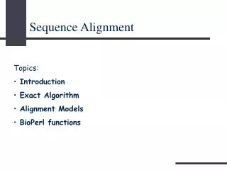
Window size Threshold window for fine tuning Dot plot window Alignment window
Set Dotlet Parameters • Dotlet slides a window along each sequence • If the windows are more similar than the threshold, Dotlet prints a dot at their intersection • You can control the similarity threshold with the little window on the left Window size Window Size Threshold Threshold
Window size Threshold window for fine tuning Dot plot window Alignment window
The Dotlet Threshold • Every dot has a score given by the window comparison • When the score is • Below threshold 1 black dot • Between thresholds 1 and 2 grey dot • Above threshold 2 white dot • The blue curve is the distribution of scores in the sequences • The peak most common score, • Most common less informative Log curve
Window size Threshold window for fine tuning Dot plot window Alignment window
Getting Your Dot Plot Right • Window size and the stringency control the aspect of your dot plot • Very stringent = clean dot plot, little signal • Not stringent enough = noisy dot plot, too much signal • Play with the threshold until a usable signal appears
Which Size for the Window? • Long window • Clean dot plots • Little sensitivity • Short window • Noisy dot plots • Very sensitive • The size of the window should be in the range of the elements you are looking for • Conserved domains: 50 amino acids • Transmembrane segments: 20 amino acids • Shorten the window to compare distantly related sequences
Window size Threshold window for fine tuning Dot plot window Alignment window
Looking at Repeated Domains with Dotlet • The square shape is typical of tandem repeats • The repeats are not perfect because the sequences have diverged after their duplication
Comparing a Gene and Its Product • Eukaryotic genes are transcribed into RNA • The RNA is then spliced to remove the introns’ sequences • It may be necessary to compare the gene and its product • Dotlet makes this comparative analysis easy
Aligning Sequences • Dotlet dot plots are a good way to provide an overview • Dot plots don’t provide residue/residue analysis • For this analysis you need an alignment • The most convenient tool for making precise local alignments is Lalign
Lalign and BLAST • Lalign is like a very precise BLAST • It works on only two sequences at a time • You must provide both sequences
LaLign http://www.ch.embnet.org/software/LALIGN_form.html
Lalign Output • Lalign produces an output similar to the alignment section of BLAST • The E-value indicates the significance of each alignment • Low E-value good alignment
Going Farther • If you need to align coding DNA with a protein, try these sites: • www.tcoffee.org => protogene • coot.embl.de/pal2nal • If you need to align very large sequences, try this site: • www.ncbi.nlm.nih.gov/blast/bl2seq/wblast2.cgi • If you need a precise estimate of your alignment’s statistical significance, use PRSS • The program is available at fasta.bioch.virginia.edu
Generalizing the Notion of Pairwise Alignment • Alignment of 2 sequences is represented as a 2-row matrix • In a similar way, we represent alignment of 3 sequences as a 3-row matrix A T _ G C G _ A _ C G T _ A A T C A C _ A • Score: more conserved columns, better alignment
Alignments = Paths in… • Align 3 sequences: ATGC, AATC,ATGC
Alignment Paths x coordinate
Alignment Paths • Align the following 3 sequences: • ATGC, AATC,ATGC x coordinate y coordinate
Alignment Paths x coordinate y coordinate z coordinate • Resulting path in (x,y,z) space: • (0,0,0)(1,1,0)(1,2,1) (2,3,2) (3,3,3) (4,4,4)
Aligning Three Sequences source • Same strategy as aligning two sequences • Use a 3-D “”, with each axis representing a sequence to align • For global alignments, go from source to sink sink