Sequence Alignment
Sequence Alignment. Lecture 2, Thursday April 3, 2003. Review of Last Lecture. Lecture 2, Thursday April 3, 2003. Sequence conservation implies function. Interleukin region in human and mouse. Sequence Alignment. AGGCTATCACCTGACCTCCAGGCCGATGCCC TAGCTATCACGACCGCGGTCGATTTGCCCGAC.


Sequence Alignment
E N D
Presentation Transcript
Sequence Alignment Lecture 2, Thursday April 3, 2003
Review of Last Lecture Lecture 2, Thursday April 3, 2003
Sequence conservation implies function Interleukin region in human and mouse Lecture 2, Thursday April 3, 2003
Sequence Alignment AGGCTATCACCTGACCTCCAGGCCGATGCCC TAGCTATCACGACCGCGGTCGATTTGCCCGAC -AGGCTATCACCTGACCTCCAGGCCGA--TGCCC--- || ||||||| |||| | || ||| ||||| TAG-CTATCAC--GACCGC--GGTCGATTTGCCCGAC Lecture 2, Thursday April 3, 2003
The Needleman-Wunsch Matrix x1 ……………………………… xM Every nondecreasing path from (0,0) to (M, N) corresponds to an alignment of the two sequences y1 ……………………………… yN Lecture 2, Thursday April 3, 2003
The Needleman-Wunsch Algorithm x = AGTA m = 1 y = ATA s = -1 d = -1 F(i,j) i = 0 1 2 3 4 Optimal Alignment: F(4,3) = 2 AGTA A - TA j = 0 1 2 3 Lecture 2, Thursday April 3, 2003
The Needleman-Wunsch Algorithm • Initialization. • F(0, 0) = 0 • F(0, j) = - j d • F(i, 0) = - i d • Main Iteration. Filling-in partial alignments • For each i = 1……M For each j = 1……N F(i-1,j) – d [case 1] F(i, j) = max F(i, j-1) – d [case 2] F(i-1, j-1) + s(xi, yj) [case 3] UP, if [case 1] Ptr(i,j) = LEFT if [case 2] DIAG if [case 3] • Termination. F(M, N) is the optimal score, and from Ptr(M, N) can trace back optimal alignment Lecture 2, Thursday April 3, 2003
The Overlap Detection variant Changes: • Initialization For all i, j, F(i, 0) = 0 F(0, j) = 0 • Termination maxi F(i, N) FOPT = max maxj F(M, j) x1 ……………………………… xM y1 ……………………………… yN Lecture 2, Thursday April 3, 2003
Today • Structure of a genome, and cross-species similarity • Local alignment • More elaborate scoring function • Linear-Space Alignment • The Four-Russian Speedup Lecture 2, Thursday April 3, 2003
Structure of a genome a gene transcription pre-mRNA splicing mature mRNA translation Human 3x10⁹ bp Genome: ~30,000 genes ~200,000 exons ~23 Mb coding ~15 Mb noncoding protein Lecture 2, Thursday April 3, 2003
Structure of a genome gene D A B C Make D If B then NOT D If A and B then D short sequences regulate expression of genes lots of “junk” sequence e.g. ~50% repeats selfish DNA gene B D C Make B If D then B Lecture 2, Thursday April 3, 2003
Cross-species genome similarity • 98% of genes are conserved between any two mammals • ~75% average similarity in protein sequence hum_a : GTTGACAATAGAGGGTCTGGCAGAGGCTC--------------------- @ 57331/400001 mus_a : GCTGACAATAGAGGGGCTGGCAGAGGCTC--------------------- @ 78560/400001 rat_a : GCTGACAATAGAGGGGCTGGCAGAGACTC--------------------- @ 112658/369938 fug_a : TTTGTTGATGGGGAGCGTGCATTAATTTCAGGCTATTGTTAACAGGCTCG @ 36008/68174 hum_a : CTGGCCGCGGTGCGGAGCGTCTGGAGCGGAGCACGCGCTGTCAGCTGGTG @ 57381/400001 mus_a : CTGGCCCCGGTGCGGAGCGTCTGGAGCGGAGCACGCGCTGTCAGCTGGTG @ 78610/400001 rat_a : CTGGCCCCGGTGCGGAGCGTCTGGAGCGGAGCACGCGCTGTCAGCTGGTG @ 112708/369938 fug_a : TGGGCCGAGGTGTTGGATGGCCTGAGTGAAGCACGCGCTGTCAGCTGGCG @ 36058/68174 hum_a : AGCGCACTCTCCTTTCAGGCAGCTCCCCGGGGAGCTGTGCGGCCACATTT @ 57431/400001 mus_a : AGCGCACTCG-CTTTCAGGCCGCTCCCCGGGGAGCTGAGCGGCCACATTT @ 78659/400001 rat_a : AGCGCACTCG-CTTTCAGGCCGCTCCCCGGGGAGCTGCGCGGCCACATTT @ 112757/369938 fug_a : AGCGCTCGCG------------------------AGTCCCTGCCGTGTCC @ 36084/68174 hum_a : AACACCATCATCACCCCTCCCCGGCCTCCTCAACCTCGGCCTCCTCCTCG @ 57481/400001 mus_a : AACACCGTCGTCA-CCCTCCCCGGCCTCCTCAACCTCGGCCTCCTCCTCG @ 78708/400001 rat_a : AACACCGTCGTCA-CCCTCCCCGGCCTCCTCAACCTCGGCCTCCTCCTCG @ 112806/369938 fug_a : CCGAGGACCCTGA------------------------------------- @ 36097/68174 “atoh” enhancer in human, mouse, rat, fugu fish Lecture 2, Thursday April 3, 2003
The local alignment problem Given two strings x = x1……xM, y = y1……yN Find substrings x’, y’ whose similarity (optimal global alignment value) is maximum e.g. x = aaaacccccgggg y = cccgggaaccaacc Lecture 2, Thursday April 3, 2003
Why local alignment • Genes are shuffled between genomes • Portions of proteins (domains) are often conserved Lecture 2, Thursday April 3, 2003
The Smith-Waterman algorithm Idea: Ignore badly aligning regions Modifications to Needleman-Wunsch: Initialization: F(0, j) = F(i, 0) = 0 0 Iteration: F(i, j) = max F(i – 1, j) – d F(i, j – 1) – d F(i – 1, j – 1) + s(xi, yj) Lecture 2, Thursday April 3, 2003
The Smith-Waterman algorithm Termination: • If we want the best local alignment… FOPT = maxi,j F(i, j) • If we want all local alignments scoring > t For all i, j find F(i, j) > t, and trace back Lecture 2, Thursday April 3, 2003
Scoring the gaps more accurately (n) Current model: Gap of length n incurs penalty nd However, gaps usually occur in bunches Convex gap penalty function: (n): for all n, (n + 1) - (n) (n) - (n – 1) (n) Lecture 2, Thursday April 3, 2003
General gap dynamic programming Initialization: same Iteration: F(i-1, j-1) + s(xi, yj) F(i, j) = max maxk=0…i-1F(k,j) – (i-k) maxk=0…j-1F(i,k) – (j-k) Termination: same Running Time: O(N2M) (assume N>M) Space: O(NM) Lecture 2, Thursday April 3, 2003
Compromise: affine gaps (n) (n) = d + (n – 1)e | | gap gap open extend To compute optimal alignment, At position i,j, need to “remember” best score if gap is open best score if gap is not open F(i, j): score of alignment x1…xi to y1…yj if xi aligns to yj G(i, j): score if xi, or yj, aligns to a gap e d Lecture 2, Thursday April 3, 2003
Needleman-Wunsch with affine gaps Initialization: F(i, 0) = d + (i – 1)e F(0, j) = d + (j – 1)e Iteration: F(i – 1, j – 1) + s(xi, yj) F(i, j) = max G(i – 1, j – 1) + s(xi, yj) F(i – 1, j) – d F(i, j – 1) – d G(i, j) = max G(i, j – 1) – e G(i – 1, j) – e Termination: same Lecture 2, Thursday April 3, 2003
To generalize a little… … think of how you would compute optimal alignment with this gap function (n) ….in time O(MN) Lecture 2, Thursday April 3, 2003
Bounded Dynamic Programming Assume we know that x and y are very similar Assumption: # gaps(x, y) < k(N) ( say N>M ) xi Then, | implies | i – j | < k(N) yj We can align x and y more efficiently: Time, Space: O(N k(N)) << O(N2) Lecture 2, Thursday April 3, 2003
Bounded Dynamic Programming Initialization: F(i,0), F(0,j) undefined for i, j > k Iteration: For i = 1…M For j = max(1, i – k)…min(N, i+k) F(i – 1, j – 1)+ s(xi, yj) F(i, j) = max F(i, j – 1) – d, if j > i – k(N) F(i – 1, j) – d, if j < i + k(N) Termination: same Easy to extend to the affine gap case x1 ………………………… xM y1 ………………………… yN k(N) Lecture 2, Thursday April 3, 2003
Introduction: Compute the optimal score F(i,j) It is easy to compute F(M, N) in linear space Allocate ( column[1] ) Allocate ( column[2] ) For i = 1….M If i > 1, then: Free( column[i – 2] ) Allocate( column[ i ] ) For j = 1…N F(i, j) = … Lecture 2, Thursday April 3, 2003
Linear-space alignment To compute both the optimal score and the optimal alignment: Divide & Conquer approach: Notation: xr, yr: reverse of x, y E.g. x = accgg; xr = ggcca Fr(i, j): optimal score of aligning xr1…xri & yr1…yrj same as F(M-i+1, N-j+1) Lecture 2, Thursday April 3, 2003
Linear-space alignment Lemma: F(M, N) = maxk=0…N( F(M/2, k) + Fr(M/2, N-k) ) M/2 x F(M/2, k) Fr(M/2, N-k) y k* Lecture 2, Thursday April 3, 2003
Linear-space alignment Now, using 2 columns of space, we can compute for k = 1…M, F(M/2, k), Fr(M/2, k) PLUS the backpointers Lecture 2, Thursday April 3, 2003
Linear-space alignment Now, we can find k* maximizing F(M/2, k) + Fr(M/2, k) Also, we can trace the path exiting column M/2 from k* Conclusion: In O(NM) time, O(N) space, we found optimal alignment path at column M/2 Lecture 2, Thursday April 3, 2003
Linear-space alignment • Iterate this procedure to the left and right! k* N-k* M/2 M/2 Lecture 2, Thursday April 3, 2003
Linear-space alignment Hirschberg’s Linear-space algorithm: MEMALIGN(l, l’, r, r’): (aligns xl…xl’ with yr…yr’) • Let h = (l’-l)/2 • Find in Time O((l’ – l) (r’-r)), Space O(r’-r) the optimal path, Lh, at column h Let k1 = pos’n at column h – 1 where Lh enters k2 = pos’n at column h + 1 where Lh exits • MEMALIGN(l, h-1, r, k1) • Output Lh • MEMALIGN(h+1, l’, k2, r’) Lecture 2, Thursday April 3, 2003
Linear-space Alignment Time, Space analysis of Hirschberg’s algorithm: To compute optimal path at middle column, For box of size M N, Space: 2N Time: cMN, for some constant c Then, left, right calls cost c( M/2 k* + M/2 (N-k*) ) = cMN/2 All recursive calls cost Total Time: cMN + cMN/2 + cMN/4 + ….. = 2cMN = O(MN) Total Space: O(N) for computation, O(N+M) to store the optimal alignment Lecture 2, Thursday April 3, 2003
The Four-Russian AlgorithmA useful speedup of Dynamic Programming
Main Observation xl’ xl Within a rectangle of the DP matrix, values of D depend only on the values of A, B, C, and substrings xl...l’, yr…r’ Definition: A t-block is a t t square of the DP matrix Idea: Divide matrix in t-blocks, Precompute t-blocks Speedup: O(t) yr B A C yr’ D t Lecture 2, Thursday April 3, 2003
The Four-Russian Algorithm Main structure of the algorithm: • Divide NN DP matrix into KK log2N-blocks that overlap by 1 column & 1 row • For i = 1……K • For j = 1……K • Compute Di,j as a function of Ai,j, Bi,j, Ci,j, x[li…l’i], y[rj…r’j] Time: O(N2 / log2N) times the cost of step 4 Lecture 2, Thursday April 3, 2003
The Four-Russian Algorithm Another observation: ( Assume m = 1, s = 1, d = 1 ) Two adjacent cells of F(.,.) differ by at most 1. Lecture 2, Thursday April 3, 2003
The Four-Russian Algorithm xl’ xl Definition: The offset vector is a t-long vector of values from {-1, 0, 1}, where the first entry is 0 If we know the value at A, and the top row, left column offset vectors, and xl……xl’, yr……yr’, Then we can find D yr B A C yr’ D t Lecture 2, Thursday April 3, 2003
The Four-Russian Algorithm xl’ xl Definition: The offset function of a t-block is a function that for any given offset vectors of top row, left column, and xl……xl’, yr……yr’, produces offset vectors of bottom row, right column yr B A C yr’ D t Lecture 2, Thursday April 3, 2003
The Four-Russian Algorithm We can pre-compute the offset function: 32(t-1) possible input offset vectors 42t possible strings xl……xl’, yr……yr’ Therefore 32(t-1) 42t values to pre-compute We can keep all these values in a table, and look up in linear time, or in O(1) time if we assume constant-lookup RAM for log-sized inputs Lecture 2, Thursday April 3, 2003