Hubs, Bridges, Switches

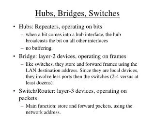
1. Hubs, Bridges, Switches • Hubs: Repeaters, operating on bits • when a bit comes into a hub interface, the hub broadcasts the bit on all other interfaces • no buffering. • Bridge: layer-2 devices, operating on frames • like switches, they store and forward frames using the LAN destination address. Since they are local devices, they involve less ports then the switches (2-4 versus at least dozens). • Switch/Router: layer-3 devices, operating on packets • Main function: store and forward packets, using the network address.

2. Network Design • Hub-based network? • Limitations: • Heterogeneity requires buffering • Collision Domain (=>Bandwidth sharing) • Ethernet limitations on number of hosts, distance etc. • Bridges can break the collision domain • Filtering, storing, forwarding • LAN addresses are not common: IP addresses are. • This is where a switch/router comes into play.

3. Comparison • Criteria • Filtering traffic - targeting the destination only (or the destination network) • collision domain • Scalable Internetworking • Store and Forward • Buffers and destination address • Routing • Tables and routing protocols • Number of ports • Location and routing protocols

4. Bridges • Early days: Transparent Bridges • Learning Bridges - small LANs • Everything goes by until the table of host/network is built • Learning Bridges - extended LANs with loops • break loops

5. Finding the node location • Forward a message to Destination D only if D is in the other portion of the network • a-b-c{<->bridge<->}d-e • Option first: • A human creates a table with the nodes and networks • Or, • The bridges look at the source ID of all frames • Records that frame from host A received on port 1 • It then builds a table such as: • a - 1 • b - 2 • c -1 • d -2 • e -2

6. Spanning Tree • Used in Extended Lans • Avoids loops due to • Redundant paths for reliability • Lack of centralized control • Provides • back-up in case of failure • dynamic configuration • Filters out remote/local traffic from local/remote networks

7. Example A B B3 C B5 B7 D B2 E F B1 G H B6 B4 I

8. Key issues • How to find the root? • How does a bridge know that is not the designated bridge? • Root and designated bridges • not a designated bridge if it receives a message from a bridge that is • closer to the root • or, equally close to the root but has smaller ID • better “root configuration message” if: • smaller ID • equal ID but shorter distance • equal ID and distance but smaller sending bridge ID

9. Protocol • Find the root • All bridges claim to be the root by sending m(bid, rid, #hops) • Bridges find out if they are designated bridges or not • They stop sending “claim” messages as soon as they discover they are not the root • They keep forwarding messages (and add 1 to #hops), as soon as they discover they are not the root • They stop forwarding as soon as they discover they not designated bridges

10. A B B3 C B5 B7 D B2 E F B1 G H B6 B4 I Example B3: M(b2, 0, b2)=> accepts B2 as root and send to B5: M(B3, 1, B2). Similarly B2 and in general Bi accepts B1 as root. B6: receives m(B4, 1, B1) from B4 (port #2), compares with (B6, 1, B1) and decides that is *not* a designated bridge. It then stops forwarding to that port Finally, B3’s both ports are going idle, B6’s both ports are going idle and B7’s upper port is going idle.

11. Switching and Forwarding

12. Inside a Switch • Input Ports • physical:terminate the incoming physical link to the router • data-link: reconstruct frame • lookup, forwarding, queuing, so that a packet is directed into the appropriate outport • control packets (e.g. RIP etc. are forwarded to the routing processor) • Switching Fabric • a network itself, connects physically input/output ports • Output Ports • As the input, in reverse order • Routing Processor • executes the routing protocols, maintains routing tables, performs network management functions

13. Router Architecture • Generic router architecture Fabric Input Port Output Port Routing Processor

14. Where does Queuing occur? • Packet queues can grow at both the input and the output ports • Suppose: • input speed = output speed • n input ports and n output ports • scenarios • all receive similar traffic and fabric has n times the speed of the port • all packets go to the same output port

15. In/Out-port Queuing • A packet scheduler at the output port must choose one packet for transmission (from the queue). For example, FIFO, WFQ etc. • Contention: • Head-of-the-line Blocking

16. Issues on source routing • Limitations • Topology has to be known • Failures or updates cannot be incorporated • Advantages • Enables path selection according to user criteria • Enables avoidance of routing protocols • Enables predetermined virtual circuits

17. Virtual Circuit Switching • Explicit connection setup (and tear-down) phase • Subsequent packets follow same circuit • Analogy: phone call • Sometimes called connection-oriented model • Each switch maintains a VC table.

18. Protocol • Two components: Signaling and Forwarding • Destination address • VCI unique for the link • VC Tables • Incoming Interface • Virtual Circuit Identifier (VCI) • Outgoing Interface • Outgoing VCI

19. Virtual Circuit • Sender A sends to port 2 a packet with VCI 5. Switch checks VCI and forwards further to outport 1 with VCI 11. Port 3 checks VCI and forwards to port 0 - out VCI = 7. The process goes on until we reach B. • Switch 1 “thinks”: Here is a packet to my input port 2 with VCI 5 (checks table...) send it to port 1 and assign a VCI 11. Switch 2 “thinks”: Here is a packet with VCI 2 at my input port 3 - send it to port 0 and assign it a VCI 7. Note: B address is not needed in the forwarding process.

20. Deciding on VCIs • Signaling • A sends packet to port 2 (from B address) • S1 receives connection request from A in port 2. • S1 creates a new entry in the table: InVCI 5, In port 2, Out port 1, OutVCI ? • S2 receives packet and assign a VCI unique for the port (11) • S2 creates entry: InVCI 11, InPort 3, Outport 0, OutVCI? • S3 similar • Host B picks up In VCI and accepts. Reply contains VCI #. S3 completes its table and send back to S2. S2 completes its table and sends back to S1. S1 back to host.

21. VCI and forwarding • VCI unique for the link, selected by the destination switch which knows what numbers are assigned already. • VCI cancels the need for B address. • B address is needed initially (at signaling) to reach the destination. • Tables are created at request stage (forward path) and completed during the response stage (reverse path) • Resource allocation can be arranged during signaling - if not enough resources request is not approved. QoS is better approached.

22. Datagrams • No connection setup phase • Each packet forwarded independently • Analogy: postal system • Sometimes called connectionless model • Each switch maintains a forwarding (routing) table

23. Protocol • Each switch keeps a forwarding table with entries Destination, port • Creating and updating dynamically the table is a subject matter of routing. Once you know the topology, you create the forwarding tables. • Information Structure. • Example Switch 2 • Destination - Port • A - 3 • B - 0 • C - 3 • D - 3

24. Virtual Circuit versus Datagram Virtual Circuit Model: • Typically wait full RTT for connection setup before sending first data packet. • While the connection request contains the full address for destination, each data packet contains only a small identifier, making the per-packet header overhead small. • If a switch or a link in a connection fails, the connection is broken and a new one needs to be established. • Connection setup provides an opportunity to reserve resources.

25. Datagram Model: • There is no round trip time delay waiting for connection setup; a host can send data as soon as it is ready. • Source host has no way of knowing if the network is capable of delivering a packet or if the destination host is even up. • Since packets are treated independently, it is possible to route around link and node failures. • Since every packet must carry the full address of the destination, the overhead per packet is higher than for the connection-oriented model.

26. 4 1 3 Host 2 Port 4 Switch 3 1 VCI 5 4 2 3 1 3 4 2 1 3 7 2 9 Source Destination

27. Routing

28. Routing • Local and global • Distinguished by their goal • Find best route / find some route • Avoid loops • Two approaches for local routers • Distance Vector • Link State

29. Notes on routing • Routing and Forwarding • Routing and Forwarding Tables • Routing associated with costs - it becomes an optimization problem • Routing is associated with overhead • Routing is associated with loops and stability • Simple routing is desirable when complexity is increased

30. Discovering the topology • Two approaches: • Send your complete table of network topology to your neighbors; they will update their tables and send updated tables to their neighbors. • Send information about your neighbors to all nodes. All collected pieces of information will be reconstructed at each node. • The first is a step-by-step construction of the topology • The second is a two step process: first collect all data, then construct the tables

31. Distance Vector (RIP) • Network as a graph • Example: A to D B A C D E F G

32. PROCEDURE • Each node constructs a one-dimensional array (vector) with the distances (costs) to all other nodes • Each table is of the form: • Destination-Cost-NextHop • Each node knows only the cost for the directly connected neighbors. • Each node distributes the vector to its neighbors • Each node calculates the best costs and decides upon final entries • No centralized authority has complete knowledge of all nodes’ tables

33. Distance Vector: Example Table • A 0 1 1 oo 1 1 oo • B 1 0 1 oo oo oo oo • C 1 1 0 1 oo oo oo • D oo oo 1 0 oo oo 1 • E 1 oo oo oo 0 oo oo • F 1 oo oo oo oo 0 1 • G oo oo oo 1 oo 1 0 • ----------------------------------------------------------------------------- • A 0 1 1 2 1 1 2 • B 1 0 1 2 2 2 3 • C 1 1 0 1 2 2 2 • D 2 2 1 0 3 2 1 • E 1 2 2 3 0 2 3 • F 1 2 2 2 2 0 1 • G 2 3 2 1 3 1 0

34. Routing Table of node A • Initial table • D/C/Next-hop • B 1 B • C 1 C • D oo - • E 1 E • F 1 E • G oo -

35. Note: • Each node sends the vector to its directly connected neighbors - not to all the nodes in the network (which does not know anyway) • Neighbors recalculate and send to their neighbors • In another approach (OSPF) nodes discover the topology first and then each node builds a table with *all* nodes • The difference in this approach is that the original vectors are forwarded without recalculation - so we consider that each node sends info to all nodes

36. Discussion • Convergence: System stabilizes • Periodic update (30 sec) • Triggered update • Link Failure • Loops • Split horizon • Split horizon with poison reverse

37. Distance Vector: Loops B A • link from A to E goes down. A advertises oo to E but B and C advertise a distance of 2 to E. B hears that E can be reached from C in two hops and concludes that can reach E through C in 3 hops. A learns that from B; it concludes that it can reach E in 4 hops and advertises to C; C advertises 5 hops... C D E F G

38. Solutions • Consider a max number of hops (cost) - when this is exceeded, restart. • Don’t send information you learned from a neighbor back to that neighbor. For example, if the entry for B is (E, 2, A) this means B has that probably from A • Or, send back a large cost • Or, wait (B and C) for sometime after hearing a failure - don’t let the others know immediately. In this case you will know that the other nodes do not really have a path • Why? B and C should get an update if there is another path - else they will not. Waiting here enables a ruling as to whether the information is current or not.

39. Link State (OSPF) • Link State Packets(LSP) • ID of the node that created the LSP • A list of directly connected neighbors and the associated costs to each one • A sequence number • Time To Live (TTL) • I am D, I can reach C at a cost of 2 and B at a cost of 3, my SN is 10 and my TTL is 5 • 1,2 -> route calculation; 3,4->process reliability

40. Reliable Flooding • All nodes create LSPs and send it to neighbors. • All nodes forward the LSPs they receive to their (new) neighbors (changing the TTL field) • All nodes receive all LSPs of the nodes; they now need to put all pieces together and make up the table.

41. Flooding Example • Nodes don’t send LSP’s back...

42. Dijkstra’s Shortest Path • M={s} • for each n in N-{s} • C(n)=l(s,n) • while (N and M not equal) • M= M {w} such that C(w) is the minimum for all w in (N-M) • for each n in (N-M) • C(n) = min (C(n), C(w)+l(w, n))

43. Justification • We start with M containing this node s and we initialize the table of costs (C(n)) to other nodes, with our directly connected neighbors • We look for the node that is reachable at the lowest cost and we add it to M. • We consider the costs of reaching nodes through w and we update the table of costs • We choose a route that goes through w if this has lower cost • We repeat the procedure until all nodes are incorporated into M • The idea is to determine lower costs for paths - then we construct the routes to destinations based on these costs.

44. Route Calculation (forward search) • Each node collects the LSPs and follows these steps: • Creates a table with fields: Step, Confirmed, Tentative • then do: • Initialize the Confirmed List with an entry for myself (cost 0) • Select neighbors’ LSPs; add them into the Tentative list • Find lower cost and put it into the Confirmed List • If tentative list is empty, stop; else, add neighbors of last entry in the confirmed list. • Continue until Tentative list is empty

45. Example for D 5 B • Confirmed - Tentative - Comment • D, 0, - / /look at D’s LSP • (D, 0, -)/ B, 11, B - C,2,C / D’s LSP says we can reach B and C (put in tentative) • D,0,1 - C,2,C/ B,11,B/Put C in confirmed; examine C’s LSP • same/B, 5, C - A, 12, C / B goes to confirm • D - C - B/ A,12,C/Check LSP of B • D - C - B - A 3 A 10 C 11 D 2

46. Metrics • Link Congestion? • Number of Hops? • Delay or Bandwidth? • Multihop consideration: resource usage. • You bother less applications