Graph Theory in Networks
302 likes | 709 Vues
Graph Theory in Networks. Lecture 4, 9/9/04 EE 228A, Fall 2004 Rajarshi Gupta University of California, Berkeley. Plan for Graph Segment. Lecture 3 – Tue (Sep 7, 2004) Paths and Routing Cycles and Protection Matching and Switching Lecture 4 – Thu (Sep 9, 2004) Coloring and Capacity

Graph Theory in Networks
E N D
Presentation Transcript
Graph Theory in Networks Lecture 4, 9/9/04 EE 228A, Fall 2004 Rajarshi Gupta University of California, Berkeley
Plan for Graph Segment • Lecture 3 – Tue (Sep 7, 2004) • Paths and Routing • Cycles and Protection • Matching and Switching • Lecture 4 – Thu (Sep 9, 2004) • Coloring and Capacity • Trees and Broadcast, Multicast • Lecture 5 – Tue (Sep 14, 2004) • Complete example: Capacity in Ad-Hoc Networks • Lectures 9 & 10 • Student Presentations (have you signed up ?)
Map coloring: Color all countries on a map using fewest colors Model: Each country is a node, edge if share boundary This forms a planar graph (edges don’t intersect) Coloring: History
Graph Planarity • Question in last class: How do I tell if graph is planar? • Kuratowski’s Theorem: A graph is planar if and only if it has no subgraph homeomorphic to K5 or K3,3 (See proof in Harary Thm 11.13) • Homeomorphic graphs: Can be obtained by sequence of subdivision of lines • K3,3: Complete bipartite graph with 3 nodes each • Can be checked in O(n3)
Five color theorem: Every planar graph is 5-colorable Heawood, 1890 Four Color Theorem: Every planar graph is 4-colorable Conjectured for many years (since 1890) Proved by Appel and Haken (1977) Can do no better than 4 colors K4 (complete graph in 4 vertices) is planar 4 & 5 Color Theorems
Lemma: In a planar graph, node w deg5 Recall Euler’s Formula v-e+f=2 A planar graph with outside face = polyhedron Let d be avg node deg. So dv=2e r be avg face deg. So rf=2e Rewrite Euler But r3, So Replacing e=dv/2, Hence For a finite graph, there must exist some node with degree < 6 f4 f1 f2 f3 5 Color Theorem (Lemma) v=4 e=6 f=4
Induction: If v<6, trivial Assume true for v-1 vertices In G, remove node v with deg<6 Color rest of graph with 5 colors Can do this due to induction hypothesis 5 Color Theorem Proof • Consider v • Look at the 5 nodes around it • If use < 4 colors, we are done
Else look at induced subgraph only with colors red and blue If v1 and v3 not connected, interchange colors of v1-component s.t v1 is colored blue. And give red color to v. Else: v1-v-v2-v1 topologically separates v2 from v4 Now repeat the procedure for v2 and v4 There cannot be path from v2 to v4 (with colors green and pink) since graph is planar Hence can change color of v2 5 Color Theorem Proof (contd)
Chromatic Number • Chromatic number • Fewest number of colors required to color a graph • Few common graphs • Kn is n-colorable • Bipartite graphs are 2-colorable • Planar graphs are 4-colorable
(max degree) • Proof by algorithm • Let the colors be 1,2,…k, where (k=1+) • For node i = 1 to N • Pick the smallest color not used by any neighbor of i • Proof • Suppose no such color exists for node i • Neighbors of i have used up all k colors • i has at least k neighbors • deg(i) k > • [Contradiction]
‘’ Direction Proof by contradiction Assume odd cycle exists Color nodes on odd cycle as R, B, R, B … Eventually last node will have two neighbors with opposite colors ‘’ Direction Take any point v Make two sets V1 and V2 V1 = nodes odd dist from v V2 = nodes even dist frm v Claim: Every edge joins V1 to V2 Suppose line xy joins two nodes in same set {v…x} and {y…v} are both odd or both even Then cycle {v…x}+{xy}+{y…v} is odd By claim, color V1red and V2blue Theorem: Graph bi-colorable iff no odd cycles
Set of nodes that do not have an edge between them Set of nodes that can have the same color Maximal IS: not contained in any other IS Result: Number of maximal IS in a graph is exponential Graph coloring algorithms find IS Finding the chromatic number of a graph is NP-hard Many approximations exist Independent Sets (IS)
Greedy Algorithm Order nodes by degree Add first node to IS Discard all neighbors into a Future bin Repeat till set empty Start with future bin Correctness Are the sets generated independent ? Are they maximal ? Complexity Each iteration adds one node, so O(m) Discarding neighbors O(n) Total: O(mn) Followup: How far is this from optimal coloring Arbitrary or Bounded Many approx algos give coloring within 4X, 6X of optimal Approximate Coloring
Vertex/Node Cover (NC) • Recall Lecture Graph1: Nodes NC of G such that every edge of G has at least one node in NC • Theorem: S is NC (V-S) is IS • Proof ‘=>’ • Suppose not • Then edge with both end-points in (V-S) • Then S does not cover this edge (Contradiction) • Proof ‘<=’ • Suppose not. Let S’ be an IS but V-S’ is not a NC • Then we have an edge with both end-points not in V-S’ i.e. both end-points are in S’ • S’ is not independent (Contradiction)
Cliques • Definitions • Clique = Complete Subgraph • Maximal Clique = Clique not a subset of any other • Clique Number = size of largest clique • Observe • Each node in a clique needs a different color • So • Clique is complement of IS = 4 Maximal Cliques: ABC, BCEF, CDF
Perfect Graphs • A graph is said to be perfect when its • Chromatic Number • Clique Number • Are equal • For all induced subgraphs • Strong Perfect Graph Theorem • Chudnovsky, Robertson, Seymour, Thomas (2002) • A graph is perfect if and only if it has no odd holes or odd anti-holes • Odd-hole is a odd cycle with no chord • Odd anti-hole is complement of odd-hole
Lovasz (1972) Take a vertex v in G Add v’ s.t. v’ is neighbor to every neighbor of v If G is perfect, then G’ is perfect Proof Consider induced subgraph H’ of G’ If v’H’, then (H’)=(H’) If v’H’ but vH’, then H’ isomorphic to corres. H If v,v’H’ Consider H=H’\{v’} Since v and v’ are not connected, can give color of v to v’ (same neighbors) So (H’)= (H) Also (H’)=(H) Clique w/o v is not enlarged Clique with v is not enlarged as v and v’ not connected But (H)=(H) as G perfect Hence (H’)=(H’) and G’ is also perfect Duplication Lemma
Trees • Define a tree G=(V,E) • |V| = |E| + 1 • Connected • Terminology • Height of a tree • Depth of a node • In-degree • Out-degree • Leaves
Types of Trees Binary Tree Each non-leaf node has exactly 2 children Ternary Tree Height Balanced Tree Root chosen s.t. height is minimized All trees are Bipartite Graphs Induced Trees Formed by choosing a subset of V,E from G Rooted Tree Rooted at particular node Spanning Tree Covers every node ‘Subset Spanning Tree’ Covers every node in a chosen subset Useful Trees
Trees in Networks • Broadcast Tree • Search Trees • BFS • DFS • Spanning Tree Protocol (STP) in Bridged Networks (e.g. Ethernet) • Multicast Tree • And many, many other places …
Tree Feature Connected No cycles Removing any edge makes it disconnected Adding any edge forms a cycle Every pair of nodes has unique path Ethernet Behavior Need all LANs to talk Loops cause broadcast storms Any bridge/port failure needs recomputation Need to disable all redundant ports Guarantees path with STP Trees and Ethernet
Concrete Example • Weight balanced Spanning Tree (WBST) • Each edge has cost • e.g. 10/100/1000 Mbps • Choose spanning tree that has min difference between min and max edge cost • Want to minimize buffering requirements as packets move through the network. Also control jitter. • Complexity
Recall Spanning Tree Algos • Kruskal’s Greedy Algorithm to compute Spanning Tree • 1. Order the edges in term of weight • 2. Add lowest cost edge (provided no loops) • 3. Check if all vertices is connected • 4. If not, return to step 2 • Any search (BFS/DFS) can check for connectedness • BFS/DFS may be performed in O(m)
WBST : Algorithm • Sort edges in increasing order of weight c1<c2<…<cm • Initialize: diff = cm-c1, low = 1, high = 1 • Take Glow,high = G (V, {ci: lowihigh}) • if Glow,high is connected • if diff > (chigh – clow) • diff := chigh – clow • Remember low, high • low := low + 1 • repeat • else • high := high + 1 • repeat
WBST : Correctness • Spanning Tree exists • By checking Glow,high is connected => spanning tree must exist • Do this using DFS. Also finds the WBST • Why balanced • Keep adding low cost edges till graph connected • Then try to discard as many low cost edges • Move both ‘low’ and ‘high’ pointers to consider other ranges • Remember best diff
WBST : Complexity • In each iteration, we either increment low, or increment high • So max number of iterations = 2m • Each iteration needs to check connectedness: DFS O(m) • So entire algo is O(m2) • Think: How would we make this algorithm distributed
Lessons from this lecture • Coloring • Cliques • Independent Sets • Useful in capacity, scheduling • Trees • Bridged Networks • Used often when want to ensure unique path etc